Impedance Matching Basics: Smith Charts

This article appeared in Electronic Design and has been published here with permission.
Members can download this article in PDF format.
What you’ll learn:
- Plot complex impedances on a Smith chart.
- Determine SWR from the Smith chart.
- Determine the impedance of a load at the end of a transmission line.
- Identify impedance-matching component values from the Smith chart.
Most of you have probably heard of the Smith chart. The intimidating graph, developed by Philip Smith in 1939, is just about as bad as it looks. How he came up with this is an untold story, but he provided a solution to the complex calculations on transmission lines. And as you will find out, it’s useful for working out transmission-line problems and in designing impedance-matching circuits. If you have avoided the Smith chart in the past, here’s a primer on how to take advantage of it.
Getting Familiar with the Chart
The Smith chart is made up of multiple circles, and segments of circles arranged in a way to plot impedance values in the form of R ± jX (Fig. 1). A horizontal line through the center of the main circle represents the resistance with R = 0 at the far left of the line and infinite resistance at the far right. Resistance values are plotted on the resistance circles, all of which are tangent to one another at the far right of the resistance line. The R = 1 circle passes through the center of the R line.
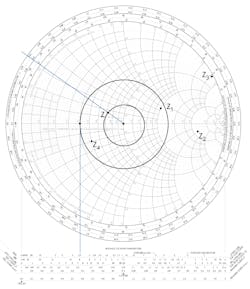
The remaining curves are parts of circles representing reactance. These curves all come together at the R = infinity point at the far right. The curves above the horizontal line represent inductive-reactance values and the curves below the line represent capacitive reactance. The Smith chart, as shown, is normalized, thereby permitting you to customize it to your application.
Plotting Values on the Chart
Figure 1 shows four examples of impedance plots:
- Z1 = 2 + j0.7
- Z2 = 6 – j2.5
- Z3 = 0.3 + j4
- Z4 = 0.5 – j0.2
Examine these examples to be sure you understand them.
To use the chart for your own work, you must first set the chart to represent values associated with a specific impedance related to your application. That impedance is usually the characteristic impedance of a transmission line you’re using or the input and output impedance of a filter or impedance-matching circuit to be created. Most RF impedances are typically 50 Ω. This value is assigned to the center of the chart where R = 1. The center point then becomes 50 Ω.
To plot a specific impedance, you must adjust it to the main impedance. To do this, you just divide the R and X values by the assigned impedance of 50 Ω, and then plot the normalized value. For example, the value of Z1 is the normalized value of 100 + j35. And Z4 is the normalized value of 25 – j10.
Additional Chart Features
Referring again to Figure 1, you will see some scales around the perimeter of the chart. These represent wavelength. The outer scale is a measure of wavelength toward the generator, the next is wavelength toward the load, and the inner scale is the reflection coefficient that’s the ratio of the reflected voltage to the incident voltage. At the bottom of the chart are scales for determining the standing wave ratio (SWR), dB loss, and reflection coefficient—all common characteristics of a transmission line.
When working with transmission lines, a main concern is the SWR. If the load is matched to the line and generator impedance, the load will absorb all of the power; there will be no reflections back to the generator. The SWR is determined with the expression:
SWR = ZL/ZO or ZO/ZL
ZL is the load impedance and ZO is the characteristic impedance of the transmission line. If ZL = ZO, then SWR = 1. This is the ideal condition so that all of the generator power gets to the load and any reflections will not interfere with the generator. The center point on the R line represents an SWR of 1. If you trace a line from that center point down so that it intersects with the SWR scale, you see that the value is 1.
If the load doesn’t match the line and the driving generator, there will be reflections back along the line. As a result, the load doesn’t receive all of the power. The SWR will be greater than 1. Assume an SWR of 2.5 is determined, which is shown as a circle on the chart (Fig. 1, again).
Around the perimeter of the chart are additional scales that represent wavelengths. One complete rotation (360 degrees) represents 0.5 wavelength at the operating frequency. One scale is called TOWARD GENERATOR and the other TOWARD LOAD.
At the bottom of the chart, the scales are SWR, reflection coefficient, and return loss.
Another Chart Version
The Smith chart also can be used with admittance (Y), susceptance (B), and conductance (G), with units in siemens (S):
- G = 1/R
- B = 1/X
- Y = 1/Z
Such a chart is a mirror image of the standard chart shown here. For some problems, the admittance version may be easier to use than the standard chart. However, Y values can be read from the standard chart, as you will see later. The best way to learn the Smith chart is to follow some examples.
Example 1
Figure 2 shows a 50-Ω generator connected to a 20-ft. piece of RG-8/U foam coax cable. The characteristic impedance of this cable is 50 Ω and its velocity factor (vf) is 0.80. Remember, the speed of a signal in a cable is slower than it is in free space. The velocity factor indicates this condition as a percentage of the speed in space. That must be considered in determining any impedance-matching solutions.
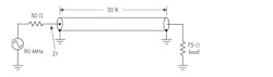
The line is terminated in a resistive load of 75 Ω. The frequency of operation is 90 MHz. With this combination, what’s the impedance that the generator sees at the cable input and what’s the SWR?
First calculate the SWR:
SWR = ZL/ZO = 75/50 = 1.5
Mark that point on the horizontal resistance line to the right of the center point. Then draw a circle around the center point through the 1.5 mark. This is the SWR circle. You can also draw a vertical line from that point down and it should intersect the SWR scale at the bottom of the chart at the 1.5 mark.
The first step is to calculate the length of the line in wavelength:
λ = 984/f
where f is in MHz:
λ = 984/90 = 10.933 ft.
We can round this to 11.
With a velocity factor of 0.8, the wavelength is:
λ = 11(0.8) = 8.8
The 20-ft. line represents:
20/8.8 = 2.27 λ
Round to 2.3 λ. Next, determine the impedance at the generator end of the line.
Starting at the 1.5 mark on the horizontal resistance line, move back toward the generator 2.3 wavelengths. Two wavelengths require four clockwise rotations. Continue to rotate another 0.3 wavelength. That’s one more half rotation (one half rotation is 0.25 wavelength) and an additional 0.3 – 0.25 = 0.05 wavelength. After that, draw a line from the 0.5 mark on the outer scale to the chart center. The point on the on the SWR circle where the line crosses is the impedance that the generator sees (Fig. 1, again):
Z = 0.67 + j0.108
Multiplying this normalized value by 50 Ω gives the actual impedance:
33.5 – j5.4
which is an inductive load.
Example 2
Assume a load impedance of 60 + j40 is connected to the 20-ft. transmission line discussed earlier. What actual impedance will the 50-Ω generator see?
Plot the load impedance on the Smith chart using the normalized value. Then divide the resistance and reactive values by 50 Ω:
1.2 + j0.8
Once you plot that value, draw the SWR circle through the impedance point. Then extend a line down vertically to the SWR scale at the bottom of the chart. The SWR is about 1.9. Now draw a line through the center point and plotted impedance so that it extends to the TOWARD GENERATOR scale on the outer perimeter.
This line intersects with the scale at 0.17. Since the generator is 2.3 wavelengths away as determined in the earlier example, you move around the circle 2.3 wavelengths. You only need to use the 0.3 value, thus you add it to the 0.17 value to get 0.47. Find that value on the TOWARD GENERATOR scale. Draw a line from the center point to the 0.47 point. The load that the generator sees is at the intersection of this line and the SWR circle. Reading from the chart you should get:
0.52 − j0.1
Multiply the normalized value by 50 to get the actual value (Fig. 3):
Z = 26 – j5
Example 3
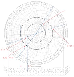
Suppose that you can measure the overall impedance of the transmission line connected to the antenna. Using an impedance bridge, SWR meter, or similar instrument, you measure a total impedance of the combined transmission line and antenna impedance that would be seen by a generator if connected. Let’s say that it is 150 + j80. We can use the same transmission line and frequency of 50 Ω and 90 MHz. The line is 2.3 wavelengths long.
Normalizing the impedance, we get:
3 + j1.6
Plot the point and draw the SWR circle. Then extend a line down to the SWR scale and read the value of 4. Next, draw a line from the center point through the plotted normalized value to the TOWARD LOAD scale on the chart perimeter. You should read about 0.273.
Now rotate in the counterclockwise direction toward the load for 2.3 wavelengths or just 0.3 as before. The intersection will be at the 0.3 + 0.273 = 0.573 or at the 0.073 mark on the TOWARD GENERATOR scale. Draw a line from the center point to that mark on the outer scale. The antenna impedance will be at the intersection of this line and the SWR circle, which is:
0.32 – j0.47
The actual value is:
Z = 16 – j23.5
If you followed this procedure, you noticed that the values are approximate since you must interpolate between the lines. It’s like reading from a slide rule, if you’re old enough to know what that is.
An Impedance-Matching Example
A well-known and useful impedance-matching technique is to use a quarter-wave matching transformer. This is a one quarter wavelength section of transmission line whose characteristic impedance (ZO) is determined by the expression:
ZO = √(ZSZL)
ZS is the source or generator impedance and ZL is the load impedance (Fig. 4).

To match a 50-Ω source (ZS) to a 100-Ω load (ZL), a quarter-wave section of transmission line is needed with an impedance of:
ZO = √(ZSZL) = √(50)(100) = √5000 = 70.7 Ω
This is a workable approach, but it has problems. First, where do you get a 70.7-Ω line? Second, if the operating frequency is in the low RF range, the line could be many feet long. Third, the impedances are purely resistive, which isn’t always the case in most applications.
However, if you are working at the higher frequencies of hundreds of megahertz or in the gigahertz range, the quarter-wave line will be short. In addition, you can create that line using microstrip or stripline on a PCB with any impedance you want by just adjusting the line widths, line spacing, dielectric material, and other factors involved in designing with microstrip lines. But other factors must be considered, such as when the source and load impedances are complex. This is where the Smith chart can be useful.
One approach to impedance matching is to use shorted transmission-line stubs in parallel with the transmission line. Figure 5 shows an example. The stub acts as a reactance to cancel out the opposite reactance at a specific point on the line as determined by the load. The objective is to find the length of the stub (l) and the distance from the load (d) where it’s to be connected.
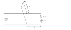
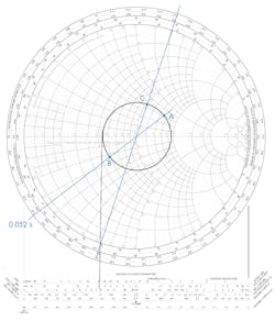
Another example will illustrate this scenario. A load impedance of ZL = 150 + j60 must be matched to a 100-Ω transmission line (Fig. 5, again) using these steps:
- Normalize the load impedance. 150/100 + j60/100 = ZL =1.5 + j0.6. Plot that on the Smith chart at point A (Fig. 6).
- Draw the SWR circle. Then draw a line down from the center of the chart to the SWR scale. It indicates an SWR of 2 to 1.
- Draw a line from the center point through point A to the perimeter of the chart and read the wavelength on the TOWARD GENERATOR scale. It is 0.052.
- Convert ZL to its equivalent admittance. This is done by noting the intersection of the line you just made from ZL through the center point to the perimeter. The point where the line crosses the SWR circle is YL. Its normalized value is YL = 0.53 – j0.23. Note the change in sign of the susceptance. This is point B in the figure.
- Move from point B clockwise around the SWR circle until it reaches the R = 1 circle on the chart. That is point C in Figure 6. This value is the normalized susceptance. B = 1 + j0.62. Draw a line from the center point through C to the perimeter. It should read 0.15 λ.
- Find the wavelength distance between the lines intersecting B and C. It is 0.15 + 0.052 = 0.202 λ. This is the distance (d) from the load to the point where the shorted line will be placed.
- The shorted stub should have the opposite susceptance of the load or −j0.62. Connecting susceptances in parallel causes them to add directly and cancel one another.
- To cancel 1 + j0.62, we need a stub that will produce 0 – j0.62. Extend the line from the 1 + j0.62 point through the center point to the R = 0 circle. Read this value on the R = 0 circle that’s the outer perimeter of the chart. Note the wavelength reading of 0.42 λ.
- Now, move from that value one quarter wavelength (0.25λ). The one quarter wavelength point gives the stub length: l = 0.42 – 0.25 = 0.17 λ.
- Now knowing the stub length and distance from the load in wavelengths, you can calculate the actual lengths at the desired operating frequency.
It’s important to point out that these values are frequency-dependent. The calculations are for a single frequency. If the line is operated over a wider range of frequencies, there will be some reflections on the line and a higher SWR.
There are other ways to perform impedance matching on a Smith chart. These procedures require the use of the chart’s admittance version as well as the standard chart used here.
Conclusion
The Smith chart is a daunting tool. If you followed the examples here, you get the picture. The chart does help to avoid some calculations, but it takes time to master it. If you work enough problems, you will become more adept at using it. Multiple online tutorials and articles can provide additional examples that will show you other ways to use the chart. To find blank Smith charts, search for downloadable charts online; there’s a variety of sources.
In addition, you should get yourself a good magnifying glass as the labels and numerical values are tiny and hard to read. A drafting compass also is needed to draw those perfect SWR circles. That will improve the accuracy in reading values from the chart.
Finally, keep in mind that there are multiple sources of Smith chart calculators and software. Most RF CAD software packages include them. Today, though, you may want to just plug in the numbers and let the computer do the work.
“Smith” is a registered trademark of the Analog Instruments Company, P.O. Box 950, New Providence, NJ 07974, 908-464-4214.
References
Bowick, B., Blyler, J., Ajluni, C., RF Circuit Design, Newnes, 2008.
Frenzel, L., Principles of Electronic Communication Systems, McGraw Hill, 2016.
Maxim Integrated Products, Application Note 742, “Impedance Matching and the Smith Chart: the Fundamentals,” 2001.
About the Author
Lou Frenzel
Technical Contributing Editor
Lou Frenzel is the Communications Technology Editor for Electronic Design Magazine where he writes articles, columns, blogs, technology reports, and online material on the wireless, communications and networking sectors. Lou has been with the magazine since 2005 and is also editor for Mobile Dev & Design online magazine.
Formerly, Lou was professor and department head at Austin Community College where he taught electronics for 5 years and occasionally teaches an Adjunct Professor. Lou has 25+ years experience in the electronics industry. He held VP positions at Heathkit and McGraw Hill. He holds a bachelor’s degree from the University of Houston and a master’s degree from the University of Maryland. He is author of 20 books on computer and electronic subjects.
Lou Frenzel was born in Galveston, Texas and currently lives with his wife Joan in Austin, Texas. He is a long-time amateur radio operator (W5LEF).
