A Review of RF Sampling vs. Zero-IF Radio Architectures

Members can download this article in PDF format.

What you’ll learn:

The choice of an RF architecture impacts how a radio will handle co-location issues.
Numerous tradeoffs are associated with both architectures.
For optimized cost, weight, and size, the zero-IF architecture wins on multiple accounts.

The growing demand for wireless services not only challenges our limited spectral resources, but it also challenges the radio designer to select the correct radio architecture. A proper radio architecture provides solid performance, and it simplifies the circuit around the radio to minimize cost, power, and size.

In the era of increasing radio deployments, the “right” radio is tolerant of current and future wireless neighbors that might otherwise cause interference down the road. This article will examine two common radio architectures and compare the tradeoffs on how each solves the unique problem of escalating co-location issues.

A Growing Challenge—New Wireless Neighbors

When the wireless revolution began some 30 years ago, only a handful of bands existed—confined mostly below 900 MHz—and typically there was one band per country. As demand for wireless services ramped up, new bands were steadily added. Currently, 49 bands¹ are globally assigned to 5G NR alone, not counting mmWave allocations. Most of the newer spectrum is above 2.1 GHz, with bands covering 500 MHz (n78), 775 MHz (n46), 900 MHz (n77), and as high as 1200 MHz (n96).

As these new bands come online, one of the biggest challenges is how to ensure adequate receiver performance in the presence of blockers in these legacy bands. This comes mainly from the co-location requirements where they’re deployed, with bands 2, 4, and 7 in the U.S., and their counterparts, bands 1 and 3, in other regions. This is particularly critical for wideband radios servicing applications in n48 (CBRS) and any portion of n77 or n78.

Wireless demands will continue to grow in the future, and the issues with co-location and interference are always present.

Radio Designs and RF Protection and Selectivity

One of the key challenges for a receiver design is protection from signals that aren’t of interest. From the beginning, radio engineers have sought different ways to accomplish this, initially with brute-force filtering and later employing various heterodyning techniques with distributed filtering.

Over the years, three key architectures have been developed to solve these challenges: direct conversion (zero-IF), super-heterodyne (IF), and direct RF sampling. While IF sampling is popular, it will not be the focus of this article. Instead, we’ll center on comparing RF sampling and zero-IF, since these are currently the most progressive implementations in the wireless domain.

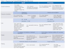
Each technique introduces different engineering tradeoffs and varying impact on the surrounding circuits and their requirements. This includes the method of frequency translation, the amount of RF and baseband gain, how RF images are dealt with, and how and where filtering is implemented. Details of these tradeoffs are shown in Table 1.

Gain Distribution and Power Dissipation

Key differences in gain distribution are prevalent between RF sampling and zero-IF. As shown in Figure 1, RF sampling has all of the gain in the RF domain given that all frequencies in the radio remain constant as the signal is processed. For comparison, Figure 2 shows a zero-IF architecture. In this architecture, part of the gain is at the RF frequency, but the balance is at baseband after the frequency translation.

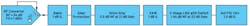
1. This diagram depicts a typical RF sampling signal chain. RF sampling has all of the gain in the RF domain, given that all frequencies in the radio remain constant as the signal is processed.

2. Represented here is a typical zero-IF signal chain. For this architecture, part of the gain is at the RF frequency, but the balance is at baseband after the frequency translation.

There are tradeoffs to both architectures. From a gain perspective, gain at higher frequencies requires more dc than lower frequencies due to the higher slew rates that are required, especially as the signals get progressively larger within the signal chain. This means that an RF sampling architecture dissipates more power in the linear RF section than does a zero-IF architecture, where a significant portion of the gain is at dc. At lower frequencies, the slew rates are lower and thus standing currents can be correspondingly less.

The challenge with RF sampling is the requirement to drive a largely capacitive input (sampling capacitor) at both high frequency and at relatively high voltage (~1 V). By contrast, a zero-IF input presents a well-behaved 50-Ω (or 100-Ω) impedance to the summing node of a baseband amplifier, which provides gain, eliminates and isolates the sample node from the RF signal, and reduces the RF drive required by the amount of gain it delivers.

That has a profound impact on power consumed in the linear RF section: It reduces the total RF dissipation by 25% to 50% in favor of zero-IF architectures by eliminating a third RF gain stage and the lower standing currents needed for baseband vs. RF amplification.

In addition to linear power is the power associated with the digitizer. With zero-IF converters, only the bandwidth required is digitized. With RF sampling, not only is a wide RF bandwidth digitized, but the sample rate far exceeds the Nyquist requirements.

Both bandwidth and sample rate are expensive in terms of power. Exact power depends on the process, but when implemented on the same process, RF converters consume about 125% more power than baseband converters for a typical single-band application. Even when two bands might be digitized by an RF converter, the power penalty is still more than 40%.

Images and Spurious Signals

Secondary tradeoffs exist in these options as well. For example, a zero-IF architecture introduces local-oscillator (LO) leakage and I/Q mismatch image terms.² On the other hand, RF sampling introduces interleave spurs³ due to mismatches within the converter architecture, as well as RF harmonics in the converter and sample-related jitter terms.⁴ The good news is that most images and spurious signals are mitigated with various background algorithms regardless of architecture.

These two architectures have vastly different frequency plans that impact the handling of aliasing and how much RF (external) filtering must be applied. Aside from architectural spurious signals, all radios will generate RF harmonics and are subject to aliasing.⁵

RF sampling radios take advantage of aliasing to downconvert the desired signal if it’s naturally beyond the first Nyquist zone. However, it’s the response of unwanted signals that are generally the issue, given that they may inadvertently fall on top of desired signals after they have been aliased. These signals must be mitigated by careful frequency planning, either by aggressive RF filtering or by sample rates that are high enough to have no aliases. Each of these comes with challenging tradeoffs.

Zero-IF architectures translate the signal to baseband (near dc). While RF harmonics are certainly created, they mix well away from the baseband in all cases and are adequately filtered by the low-pass response of the typical zero-IF input structure noted in following paragraphs. Similarly, aliasing also is mitigated by the relatively high sample rates of the baseband sampler used and the selfsame input structure.

Zero-IF Filter Requirements

One easily overlooked feature of a zero-IF architecture is that the baseband input amplifier will typically be constructed as an active low-pass filter operating as an integrated analog filter, which greatly reduces the analog filter burden. In addition to performing on-chip decimation filtering, it functions as a programmable channel filter to eliminate signals closer than those associated with Nyquist.

Furthermore, the sampling devices within zero-IF receivers often include feedback that provides additional out-of-band rejection. In effect, this means that the out-of-band regions of the radio have a larger full-scale range than the in-band regions.

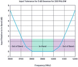
As demonstrated in previous writings⁶ and shown in simplified form in Figure 3, zero-IF radios inherently offer good tolerance to out-of-band signals. In Figure 3, the vertical axis represents the input power level relative to in-band signals that would cause a 3-dB desense, showing that in-band signals have a built-in tolerance to out-of-band signals not found in other architectures.

3. An example of the impact of on-chip zero-IF filtering, showing that zero-IF radios inherently offer good tolerance to out-of-band signals.

Because of this built-in filtering, the primary concern becomes protection of the RF front end—that is, the low-noise amplifier (LNA). A typical configuration will include a surface-acoustic-wave (SAW) filter between the first- and second-stage LNAs for frequency-division duplexing (FDD) and some time-division duplexing (TDD). Some TDD applications will integrate the SAW filter after the second stage, but the second stage can be bypassed under large input conditions (Fig. 1, again).

Typically SAW filters will provide about 25 dB of out-of-band rejection, and that’s assumed here. In addition to the SAW filter, a cavity filter is required on the antenna side of the LNA, which is shared with the transmitter.

A typical LNA might have an input 1-dB compression point of –12 dBm. If the out-of-band or co-location requirements are 16 dBm, these signals must be filtered to about 10 dB (or more) below the input 1-dB compression point of the LNA. This is a minimum of 38-dB rejection (+16 – -12 + 10). If we include the SAW filter, total out-of-band rejection is 63 dB as presented to the input of the zero-IF.

Assuming RF gain doesn’t roll off and including the total filter rejection up to the core radio input, the maximum out-of-band signal level will be –20 dBm. This is well below the typical full scale and will be further attenuated by the on-chip filtering. No spurious signals or desense would be anticipated from this input level when compared to Figure 3.

RF Sampling Filter Requirements

Two concerns arise when working with RF converters that require direct attention for filtering. First, any signal regardless of input level can create undesired spurious signals that may occupy the same frequency as the desired signal.

Spurs related to interleaving are dealt with by algorithms, but architectural spurs are another issue as they can be unpredictable. For many older RF converters, this was a constant challenge to radio performance. Fortunately, many new converters include background dither⁷ in one form or another to mitigate these issues and present relatively clean spurious-free dynamic-range (SFDR) sweeps (Fig. 4).

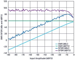
4. Today’s converters often perform background dithering to present relatively clean spurious-free dynamic-range (SFDR) sweeps.

What’s notable in this SFDR vs. input level plot is that the first 15 dB show degradation due to slew-rate limitations in the converter, which will typically generate strong second and third harmonics that must be abated. Once the RF input is below this level, harmonics and architectural spurs are typically no longer an issue (consult converter performance to verify).

With a full scale of 1 dBm, it can be expected that spurious signals will reduce significantly by the time out-of-band signals are rejected below –14 dBm into the converter. With a conversion gain of 50 dB, as shown in Table 2, this equates to –64 dBm at the antenna. If the input is potentially 16 dBm, then the RF filtering needs to be 80 dB or more for non-aliased cases.

Assuming a SAW filter provides 25 dB, this leaves 55 dB for the cavity filter to adequately protect the RF ADC from generating nonlinearities due to out-of-band signals. It also protects the input of the first-stage LNA from being driven into nonlinearity by out-of-band signals. This example represents a well-behaved converter, but the SFDR vs. input level of the converter selected should be closely examined to determine if more filtering is required.

The other concern for RF converter architectures is based on current merchant silicon, namely alias protection. Current RF converters are based on cores that operate between 3 and 6 Gsamples/s. At these low rates, it’s impossible to avoid aliased terms without the use of aggressive filtering to mitigate the impact of aliasing. This problem only abates after sample rates reach double-digit gigahertz levels.

A simplified way to consider the impact of aliasing on filter requirements is to consider the protection of a single resource element from the aliased 16-dBm co-location requirement. The goal is to suppress the aggressor to the point that should it alias to a desired rejection band, it’s filtered sufficiently so that no disruption occurs.

A wide-area reference channel based on a G-FR1-A1-4 signal would account for a signal level per rejection band of –118.6 dBm at approximately 0 dB SNR. Therefore, the offender must be filtered to 10 to 15 dB lower, or about –130 dBm, to prevent disruption. Thus, a total rejection of about 150 dB is needed, or about 125 dB from the cavity filter with one SAW filter providing the balance of filtering.

Filter Summary

Figure 5 shows the cavity filter requirements for both RF sampling and zero-IF. Because the RF sampling architecture has two separate requirements, the most restricting will dominate and a realizable filter would simply have to meet the most restrictive (125 dB) rejection to cover the entire band.

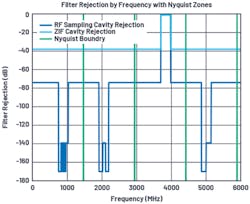
5. This plot shows the cavity filter requirements for both RF sampling and zero-IF architectures.

While such filtering is readily available, it comes at the cost of a bulky filter. In contrast to the zero-IF architecture, where only 40-dB rejection is required, the result is a significant weight and size savings given this performance is possible with a four-cavity filter.

Conclusion

Both zero-IF and RF sampling architectures provide exceptional capability. However, when the goal is optimized cost, weight, and size, the zero-IF architecture wins on multiple accounts.

From the perspective of power, the zero-IF architecture with integration of significant portions of analog gain offers a compelling power savings. Similarly, when considering the impact of filtering, zero-IF offers the potential to significantly downsize the filter requirements. While the cost differential of the filters may be small, the size and weight reduction of these filters should move beyond 50% based on the required number of cavities.

References

1. 3GPP, 38.104 Rel 16, V16.5.0, 2020-09.
2. Ashkan Mashhour, William Domino, and Norman Beamish. “On the Direct Conversion Receiver—A Tutorial.” Microwave Journal, June 2001.
3. Jonathan Harris. “The ABCs of Interleaved ADCs.” Analog Devices, Inc., October 2019.
4. Brad Brannon. “AN-756: Sampled Systems and the Effects of Clock Phase Noise and Jitter.” Analog Devices, Inc., 2004.
5. Walt Kester. “MT-002: What the Nyquist Criterion Means to Your Sampled Data System Design.” Analog Devices, Inc., 2009.
6. Brad Brannon, Kenny Man, Nikhil Menon, and Ankit Gupta. “AN-1354: Integrated ZIF, RF to Bits, LTE, Wide Area Receiver Analysis and Test Results.” Analog Devices, Inc., July 2016.
7. Brad Brannon. “AN-410: Overcoming Converter Nonlinearities with Dither.” Analog Devices, Inc.
About the Author
Brad Brannon
System Applications Engineering Director, Analog Devices Inc.
In his 37-year career at Analog Devices since graduating from North Carolina State University, Brad Brannon has held positions in design, test, applications, and system engineering. Currently, Brannon develops reference designs for O-RAN in support of those customers. He has authored several articles and application notes on topics that span clocking data converters, designing radios, and testing ADCs.