Algorithms to Antennas: Improve Radar Simulation Fidelity with Land and Sea Surface Models
This blog is part of the Algorithms to Antennas Series
What you'll learn:
- How to create land and sea surface models for monostatic radar.
- Defining regions where you want to generate clutter.
In our most recent blog, we discussed the importance of modeling radar systems at different abstraction levels. We used an automotive radar design to show how these levels of abstraction can be used consistently across different phases of the radar lifecycle.
Another important aspect of these models relates to the fidelity of the scenario being used in the simulation. For automotive radar, this typically includes the effects of multipath reflections off dynamic and static objects, which we have also written about in this series.
For radar systems that operate over broader expanses of land and sea surfaces, the fidelity of a simulated scenario is driven by how closely the scenario represents these surfaces. This is important because radar systems receive unwanted radar returns from land and sea, which are often referred to as clutter. Radar system engineers and radar signal-processing engineers are focused on removing the effects of this clutter to detect targets.
Of course, modeling land and sea surfaces supports other uses, including applications where a radar is imaging the land surface, such as synthetic aperture radars (SARs). In addition, radar systems may measure the sea state based on the returns from the waves. Radar altimeter applications are another example where the land surface also is the target, as the altimeter estimates the distance to the ground on an approach to a landing.
For all of these applications, a faithful representation of the scenario can save many hours of field testing. Furthermore, it can save time up-front during the radar installation to calibrate the system for site-specific power levels.
Monostatic Radar Models
Here, we will focus on modeling land and sea surfaces for monostatic radar applications. The modeling examples we show can be applied to both measurement-level and signal-level models. We have included several links at the end of this blog where you can learn more.
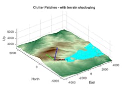
Let’s start by creating a radar scenario using terrain data from a Digital Terrain Elevation Data (DTED) file. This data can be directly imported into MATLAB to create a site-specific radar scenario (Fig. 1). The scenario visualization in Figure 1 includes a radar with a beam (represented in the cyan overlay) where the shadowed regions are omitted. Shadowing occurs where the surface is occluded due to surrounding terrain features.
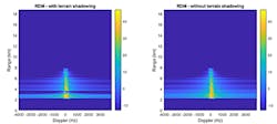
In Figure 2, you can see side-by-side range-Doppler maps for a comparison of how terrain shadowing affects the processed return. Figure 2 (left) includes the more realistic effects with shadowing, while Figure 2 (right) shows the results without shadowing. Note the gap in the left range-Doppler map that corresponds to the gap in the cyan coverage in Figure 1.
Terrain attributes can impact the scattering profile of the radar signals. For example, a rocky mountain top will return reflections that are different from those of a dense forest. When you model land and sea surfaces, you also can associate a radar reflectivity model with a specific portion of terrain.
Radar Toolbox includes 18 built-in reflectivity models, as well as support for user-specified custom reflectivity tables, which can be applied to land and sea surfaces. The range of reflectivity models helps match scenario-specific parameters, including the grazing angle and operating frequency of the radar.
Defining Regions
You can define regions on the surface where you want to generate clutter. This includes mainlobe clutter return, which is generated from the footprint of the mainlobe. You also can specify a ring-shaped region of the scenario surface within which clutter is generated for cases when the region of interest is outside the mainlobe. The region of interest can be defined by an interval in range and azimuth angle.
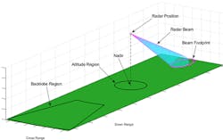
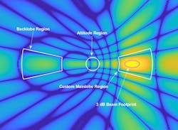
Figure 3 illustrates these two region types. The beam footprint region is displayed as a magenta ellipse where the beam intersects the ground. There are two ring regions: one directly underneath the radar for capturing an altitude return and another for capturing the backlobe clutter return.
In Figure 4, you can see how the customizable ring-shaped regions are used to capture clutter returns from arbitrary lobes of the antenna pattern.
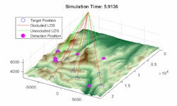
Another important reason to include terrain in a radar simulation is to account for occlusion. This is when a target isn’t in the line of sight because terrain is blocking the radar signal. Figure 5 shows a radar scanning a mountainous region. There are multiple targets on the terrain: The green lines indicate a line of sight (LOS) exists between the radar and the detection position, and the red line indicates the target is occluded.
Maritime Radar
Now that we have shown land surfaces, let’s look at maritime radar systems. Radar reflections off the surface of the sea also create a challenging and dynamic environment. To improve detection of targets of interest and assess system performance, it’s important to understand the nature of returns from sea surfaces.
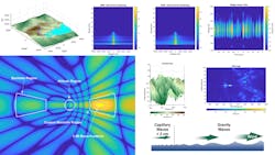
Figure 6 shows that the sea surface motion varies based on wave type and location. Capillary waves are high-frequency, small-wavelength waves with rounded crests. Gravity waves are longer, low-frequency waves. The greater the wind speed, the greater the energy transferred to the sea surface and the larger the waves. You can model a specific sea surface by defining wind direction, wind speed, and fetch—the latter is the length of water over which wind blows without obstruction.

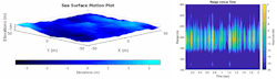
Figure 7 (left) shows the model of a sea surface as a sea state 4 with a wind speed of 19 knots. Figure 7 (right) presents a range-vs.-time plot from the corresponding signal-level simulation. Note that at a given range, the magnitude changes with time. The returns occur in a small subset of range due to the geometry (radar height, beamwidth, and depression angle).
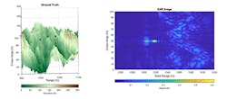
The last example we’ll discuss is a SAR system in which the terrain is part of the image generated by the radar. Figure 8 (left) shows the ground truth terrain with three targets on the land surface. In our previous discussion, we used DTED data to generate the terrain, but custom terrain data also be used. This is the case in Figure 8.
The corresponding SAR image also is illustrated in Figure 8 (right). You can see how the terrain shows up in the generated image. Note that there are two targets at the slant ranges between 1300 and 1320 meters. The third target is occluded by terrain.
Overall, the ability to model land and sea surfaces in a radar simulation can help you improve how your system will perform before it’s installed in the field. The range of radar reflectivity models that can be used with terrain and sea surfaces provides flexibility in matching the end operational environment your system will run in.
To learn more about the topics covered in this blog and explore your own designs, see the examples below or email me at [email protected].
- Introduction to Radar Scenario Clutter Simulation (Example code): Learn how to generate monostatic surface clutter signals and detections in a radar scenario.
- Simulating Radar Returns from Moving Sea Surfaces (Example): Learn to model maritime radar systems that operate in a challenging, dynamic environment, including returns from sea surfaces.
- Simulated Land Scenes for Synthetic Aperture Radar Image Formation (Example code): Learn how to simulate an L-band remote-sensing SAR system.
See additional 5G, radar, and EW resources, including those referenced in previous blog posts.
Rick Gentile is product manager, Sara James is senior software engineer, Landan Rubenstein is senior engineer, Vincent Pellissier is engineering manager, and Honglei Chen is principal engineer at MathWorks.
Read more blogs in the Algorithms to Antennas Series
About the Author
Rick Gentile
Product Manager, Phased Array System Toolbox and Signal Processing Toolbox
Rick Gentile is the product manager for Phased Array System Toolbox and Signal Processing Toolbox at MathWorks. Prior to joining MathWorks, Rick was a radar systems engineer at MITRE and MIT Lincoln Laboratory, where he worked on the development of several large radar systems. Rick also was a DSP applications engineer at Analog Devices, where he led embedded processor and system level architecture definitions for high performance signal processing systems used in a wide range of applications.
He received a BS in electrical and computer engineering from the University of Massachusetts, Amherst, and an MS in electrical and computer engineering from Northeastern University, where his focus areas of study included microwave engineering, communications, and signal processing.
