Algorithms to Antennas: Modeling a FMCW Long-Range Radar at Different Abstraction Levels
This blog is part of the Algorithms to Antennas Series
What you'll learn:
- Specifics about the system, measurement, and signal abstraction-level models.
- Applying the Radar Designer app in these scenarios.
- Results obtained from example tests, including detection locations.
In a previous blog, “Automotive Radar Modeling and Simulation,” we showed how by using a common scenario, you can build a model of an automotive radar that generates signals, detections, or tracks. We described how the level of abstraction used on a project depends on multiple factors, such as the phase of the radar development lifecycle, the length of the scenario being simulated, and the type of engineering work being performed. This same type of workflow applies to radar systems outside automotive, including surveillance radar systems.
It's important that the models across the abstraction layers have consistent results. In this blog, we’ll compare results across three abstraction levels: system-level, measurement-level, and signal-level models. For this comparison, the AWR2243 Single-Chip 76- to 81-GHz FMCW Transceiver from Texas Instruments is used as a reference design case.
Long-Range Automotive Radar Example
Our scenario is focused on a 77-GHz, long-range automotive radar. The radar uses a 26-µs pulse repetition interval and a 0.65 duty cycle, which represents the ratio of sweep time over the sweep repetition interval.
The total transmit and receive gains are calculated as the sum of the antenna element directivity (12 dBi) and the array factor (11 dB for the 12-element Tx array and 12 dB for the 16-element Rx array).
The scenario includes a mid-sized sedan, which we represent as a 10-dBsm, non-fluctuating radar cross-section (RCS) target. The goal is to detect the vehicle with a probability of 0.9 and limit false alarms to a rate of 1e-6. For simplicity, we assume environment losses are limited to free-space propagation, but it’s easy to include the effects of rain, gas, and fog to the analysis.
Using the Radar Designer App
Figure 1 shows the design parameters in the Radar Designer app, which is part of Radar Toolbox. The panel tabs shown on the left of the app are used to specify the details of the radar design, the target characteristics, and the environmental conditions.
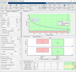
The SNR vs. range plot in Figure 1 shows the available SNR of a single sweep before any signal processing is performed in the receiver. For a target at approximately 25.4 meters, the single sweep SNR is predicted to be around 47 dB. In addition, the detectability factor charts in Figure 1 indicate that with 128 sweeps, a coherent integration gain of 21 dB is achieved. This increases the achieved SNR from 47 dB to 68 dB.
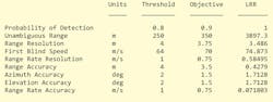
The table at the bottom of the Radar Designer app reveals that the predicted performance metrics of the design (right column) meet all threshold requirements (left column) and all objective requirements (middle column) except for the azimuth and elevation accuracy. The table below shows the metrics exported from the app that are used to help configure a measurement-level model.
Measurement-Level Model
The measurement-level model abstracts the detailed signal-processing chain. This type of model produces detections with statistics governed by the desired probabilities of detection and false alarm—they’re evaluated for a reference RCS at a reference range corresponding to the detectability threshold. The measurement-level model has additional key parameters that map to the radar configuration:
- 4-element series-fed patch azimuth field of view of 120 deg
- 4-element series-fed patch elevation field of view of 60 deg
- Required azimuth resolution of 1.4 deg
- Bandwidth of 43 MHz
With this configuration, our measurement-level radar is now configured to match the design parameters analyzed in the Radar Designer app.
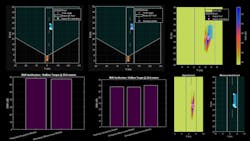
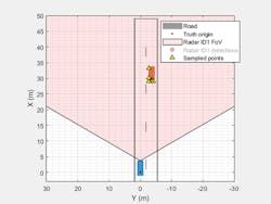
Figure 2 shows the scenario ground truth and detections generated from the measurement-level model in a bird's-eye plot.
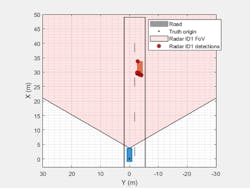
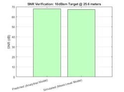
Note that the generated detections lie along the outline of the target vehicle. For the detections shown, the maximum signal-to-noise ratio (SNR) is 67.3 dB.
Figure 3 illustrates the close comparison of the SNR of the detections generated by the measurement-level radar to the system-level radar analysis performed using the Radar Designer app. For a consistent comparison, the coherent processing gain from all 128 pulses in the processing interval must be included, so we use an SNR of 68 dB from the system-level analysis in the plot.
Signal-Level Model
Using the measurement-level model, we can create an equivalent signal-level model that can simulate I/Q signals. The radar transceiver used to generate I/Q signals includes direct models for waveforms (frequency-modulated continuous wave, or FMCW, for this use case), receive and transmit antenna arrays, and other radar subsystems.
We adjust the transmitter’s peak power level to account for the beamforming gains from the transmit and receive arrays and set the noise figure to match the value used by the design in the Radar Designer app.
Radar propagation paths are generated from the target poses in the scenario. The target vehicle is modeled as an extended target using a set of point targets located along the vehicle’s extent (Fig. 4). The spacing of the point targets is determined by the azimuth and range resolution of the radar.
The signal-level model now generates baseband I/Q samples at the output of the radar receiver from the propagation paths for the target. The radar's field of view is electronically scanned by beamforming on transmit and stepping the transmit angle by the receive array’s beamwidth. Range and Doppler processing is performed for each frame of the I/Q data.
We compare the SNR of the range, Doppler, and beamformed data cube to a detection threshold. Again, the detection threshold is selected to match the desired detection probability of 0.9 and false-alarm rate of 1e-6 of our initial radar design. This results in multiple range, Doppler, and beam bins that cross the threshold level. Detection crossings are clustered using DBSCAN, which is a common algorithm used to identify threshold crossings that are likely coming from a single target.
In our example, the number of clustered detections agrees with the number of point targets employed to model the extended target. We can then estimate the range, range-rate, and azimuth angle associated with each cluster of detection threshold crossings.
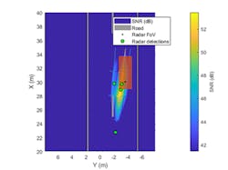
Figure 5 shows the range-angle image of the SNR values in the range, Doppler, and beamformed data cube and overlays the image with the signal-level detections extracted from the data cube.
We’re now able to find the maximum SNR from the signal-level detections, which include processing loss from the target’s range relative to the duration of the FMCW sweep. This loss can be reduced by increasing the sweep time of the FMCW waveform, but with the cost of processing more data and longer waveform transmission times.
Figure 6 shows the SNR comparison of the detections generated by the signal-level radar to the measurement- and system-level radars.
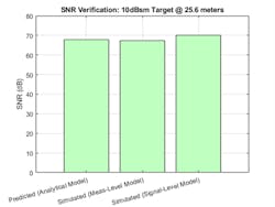
A small variation (less than 3 dB) in SNR is expected due to losses present in the signal-level model. These either aren’t included or are assumed to be constant in the measurement- and system-level models.
Signal- vs. Measurement-Level Detection Locations
Figure 7 shows the detection locations between the signal-level (left) and measurement-level (right) radars.
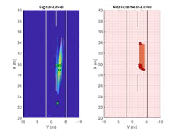
Note that both radar models generate detections that lie along the exterior of the extended target as expected, since this is in the radar’s line of sight. The number of detections between the two abstract levels varies slightly based on model fidelity and the clustering and detection algorithms that were used.
Also, while we performed signal processing that included sidelobe blanking to achieve the results shown in Figure 7 (left), an additional detection is produced close to 23 meters. This is something that can occur in long-range radars where the vehicle is detected at a close range. The ability to simulate this behavior is important to further refine your signal-processing approach without having to collect road data.
With each of the models in place, further analysis can be conducted by varying the scenario, the radar parameters, and the radar design components to match other use cases.
To learn more about the topics covered in this blog and explore your own designs, see the examples below or email me at [email protected]:
- Design and Simulate an FMCW Long-Range Radar (LRR) (example code): Learn how to design and predict performance for an FMCW long-range radar.
- Simulate Radar Ghosts Due to Multipath Return (example code): Learn how to simulate ghost target detections and tracks due to multipath reflections, where signal energy is reflected off another target before returning to the radar.
- Highway Vehicle Tracking with Multipath Radar Reflections (example): Learn to track vehicles on a highway in the presence of multipath radar reflections. Use a ghost filtering approach with an extended object tracker to simultaneously filter ghost detections and track objects.
See additional 5G, radar, and EW resources, including those referenced in previous blog posts.
Read more blogs in the Algorithms to Antennas Series
About the Author
Rick Gentile
Product Manager, Phased Array System Toolbox and Signal Processing Toolbox
Rick Gentile is the product manager for Phased Array System Toolbox and Signal Processing Toolbox at MathWorks. Prior to joining MathWorks, Rick was a radar systems engineer at MITRE and MIT Lincoln Laboratory, where he worked on the development of several large radar systems. Rick also was a DSP applications engineer at Analog Devices, where he led embedded processor and system level architecture definitions for high performance signal processing systems used in a wide range of applications.
He received a BS in electrical and computer engineering from the University of Massachusetts, Amherst, and an MS in electrical and computer engineering from Northeastern University, where his focus areas of study included microwave engineering, communications, and signal processing.
