Algorithms to Antennas: Automotive Radar Modeling and Simulation
This blog is part of the Algorithms to Antenna Series
What you'll learn:
- Building an automotive radar that generates signals, detections, or tracks.
- Higher-fidelity simulation with a radar mounted on an ego vehicle.
- Using a three-bounce path to model multipath.
- Using a physics-based model to to generate time-domain IQ signals.
We have covered a range of specific topics that relate to automotive radar system modeling and design. A couple of our most recent posts are:
This blog shows how to build a model of an automotive radar that can be used to generate signals, detections, or tracks. Radar engineers who simulate and model algorithms and systems work across a range of abstraction levels that span the RF, signal, and data-processing domains. The level of abstraction depends on the phase of the radar development lifecycle, the length of the scenario being simulated, and the type of engineering work being performed.
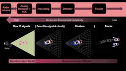
As shown in Figure 1, these different levels of abstraction range from probabilistic, measurement-level simulations based on the radar equation to physics-based models, also referred to as waveform-level models. The common theme is that the range of models can be generated using the same ground-truth scenario, which makes it easy to evaluate design tradeoffs consistently across a project and across a larger team.
At the early stages of a project, when design tradeoffs are being explored, modeling at the radar-equation level may be adequate. As a project progresses, it’s necessary to increase the level of model fidelity, moving from statistical-level to signal-level simulation. In addition, the length of a scenario can dictate which modeling abstraction level makes sense.
For example, for longer scenario times (seconds, minutes, or longer), it may be better to generate statistical or probabilistic radar detections and tracks to cover a more complex scenario or test tracking and sensor-fusion algorithms. Alternatively, higher-fidelity, physics-based simulations that include RF components, transmitted waveforms, and signals at a receive array are needed for events of interest or during development of signal-processing algorithms.
Higher-fidelity simulations also can take into account the detailed designs for the antenna array and RF subsystem, which also has been covered in our blog series. These types of simulations can be used to augment data collected on road tests.
To demonstrate the idea, we simulate a simple scenario with a radar mounted on an ego vehicle. To help make the scenario a bit more realistic, the effects of multipath propagation are added. Starting with a statistical model, we show how to generate detections and tracks based on the scenario. You will then see how to move directly to a waveform-level model to generate IQ signals using the same scenario.
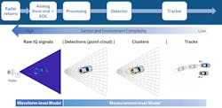
Figure 2 shows a bird’s-eye plot of the detections generated from a forward-looking automotive 77-GHz radar mounted on an ego vehicle. In addition to the vehicle in the left lane, a barrier is present at the edge of the right lane. Detections are generated by the statistical radar model for a range up to 100 meters for targets with radial speeds of up to 100 m/s. To start, we model the environment as free space for this simulation.
Note the locations of the detections along the target vehicle as well as along the side of the barrier. This type of model is good to start with, but we know that the returns from an actual system will not be so ideal.
One phenomenon that can pose considerable challenges to radar engineers is multipath. Multipath returns are present when the signal propagates directly to the intended target and back to the radar, along with reflections off other objects in the environment.
When a radar signal propagates to, and reflects back from, a target of interest, the signal can take various paths. The number of paths is unbounded, but with each reflection, the signal energy decreases. It’s common to use a three-bounce path to model this phenomenon.
To understand the three-bounce model, let’s first look at the simpler one-bounce and two-bounce paths.
The one-bounce path propagates from the radar (1) to the target (2) and then is reflected back to the radar (1). This is often referred to as the direct or line-of-sight path.
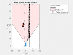
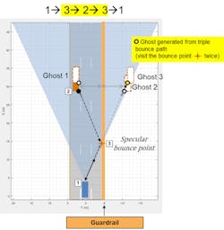
As shown in Figure 3, two unique propagation paths consist of two bounces. The first two-bounce path propagates from the radar (1) to a reflecting surface (3), then to the target (2) before returning to the radar (1). Because the signal received at the radar arrives from the last bounce from the true target, it will generate ghost detections along the same direction as the true target. Since the path length for this propagation is longer, it (shown as Ghost 1 in Figure 3) will appear at a farther range than the true target detections.
The second two-bounce path propagates from the radar (1) to the target (2), then to the reflecting surface (3) before returning to the radar (1). In this case, the ghost detections (shown as Ghost 2 in Figure 3) appear on the other side of the reflecting surface since that’s the direction the radar will receive the reflected signal.
Notice that the path length for both two-bounce paths is the same. This means the measured range and range rate for these paths will be the same as well.
As shown in Figure 4, the three-bounce path reflects off the barrier twice. This path never propagates directly to the target or directly back to the radar. The three-bounce ghost detections (shown as Ghost 3 in Figure 4) will appear on the other side of the reflecting surface, since that’s the direction the radar will receive the reflected signal. In addition, it has the longest propagation path length of the three-bounce paths and will therefore have the longest measured range of the three paths. This path corresponds to a mirror reflection of the true target on the other side of the barrier.
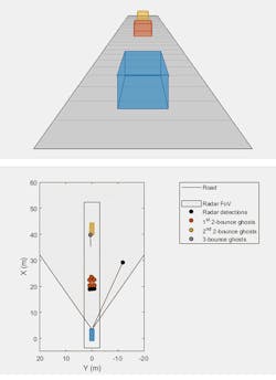
When we use multipath in our model, the results are shown in Figure 5 (top). The first two-bounce ghosts lie in the direction of the target at a slightly longer range than the direct-path detections. The second two-bounce and three-bounce detections lie in the direction of the mirrored image of the target generated by the reflection from the barrier, and at the same range as the first two-bounce.
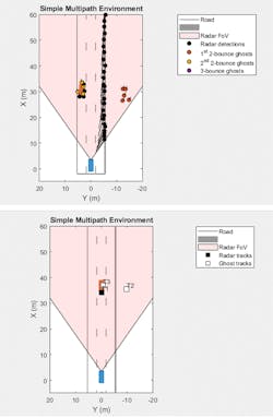
To test trackers for these types of scenarios, it’s also important to be able to generate test data without always having to collect data from road testing. The same model that generates the detections in Figure 5 (top) can be configured to directly generate tracks. Figure 5 (bottom) shows the confirmed track positions using square markers. The tracks corresponding to the barrier are not plotted.
You can see multiple tracks associated with the lead car. These tracks correspond to the true detection and the first two-bounce ghost. The tracks that lie off of the road on the other side of the guardrail correspond to the second two-bounce and three-bounce ghosts. Here, track velocities are indicated by the length and direction of the vectors pointing away from the track position (these are small because they are relative to the ego vehicle).
Ghost detections may fool a tracker because they have kinematics like those of the true targets. These ghost tracks can be problematic—they add an additional processing load to the tracker and will possibly confuse control decisions using the target tracks. For ways to handle this type of scenario, read the example Highway Vehicle Tracking with Multipath Radar Reflections.
Moving to Waveform-Level Simulations
So far, we’ve covered multipath simulations using statistical radar models to generate detections and tracks. Now, we can move to an equivalent physics-based model to generate time-domain IQ signals. The physics model is generated directly using the parameters from the statistical model. This includes the parameters we used for our 77-GHz radar above. In addition, the scenario is the same.
For the physics-based model, we integrated a linear array to the receive antenna. We can compute the three-bounce paths for the target and sensor positions from the multipath scenario. The result of the physics-based simulation is a radar data cube with three dimensions: fast-time samples, receive channels from the antenna array, and slow-time samples (collected over multiple pulses).
We first perform range and Doppler processing along the first and third dimensions of the data cube. We form beams from the receive channels along the second dimension of the data cube. Figure 6 shows the range-angle map from the beamformed, range, and Doppler processed data cube.
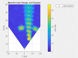
The local maxima of the received signals correspond to the location of the target vehicle, the guardrail, and the ghost image of the target vehicle on the other side of the guardrail.
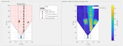
In Figure 7, you can see that statistical detections generated by the model are consistent with the peaks in the range-angle map generated from the equivalent waveform-level model using the same scenario. Note that that the two models are independent, and the observed consistency is a first validation of the statistical model.
Finally, we’re often asked whether multipath ghost detections can be used to see objects in the road that would otherwise not be detected by the radar due to occlusion. One good example of this is the detection of an occluded vehicle due to multipath off of the road surface.
With a small update to the scenario, we add a slower moving vehicle in the same lane as the ego vehicle. This slower vehicle is occluded by another vehicle directly in front of the radar as shown in the top plot of Figure 8. Note also that the side barrier has been removed for clarity, but more complex scenarios can be modeled with multipath reflections coming from all directions.
Here, the yellow car is occluded by the red car. A direct line of sight doesn’t exist between the blue ego car’s forward-looking radar and the yellow car, but multipath can pass through the space between the underside of the car and the road surface. The detection from the occluded car is possible due to the three-bounce path that exists between the road surface and the underside of the orange car.
To learn more about the topics covered in this blog and explore your own designs, see the examples below or email me at [email protected]:
- Simulate Radar Ghosts Due to Multipath Return (example code): Learn how to simulate ghost target detections and tracks due to multipath reflections, where signal energy is reflected off another target before returning to the radar.
- Highway Vehicle Tracking with Multipath Radar Reflections (example): Learn to track vehicles on a highway in the presence of multipath radar reflections. Use a ghost filtering approach with an extended object tracker to simultaneously filter ghost detections and track objects.
- Automotive Radar Design (documentation): Learn to develop probabilistic and physics-based radar sensor models, simulate MIMO antennas, waveforms, I/Q radar signals, micro-Doppler signatures, detections, clusters, and tracks.
See additional 5G, radar, and EW resources, including those referenced in previous blog posts.
About the Author
Rick Gentile
Product Manager, Phased Array System Toolbox and Signal Processing Toolbox
Rick Gentile is the product manager for Phased Array System Toolbox and Signal Processing Toolbox at MathWorks. Prior to joining MathWorks, Rick was a radar systems engineer at MITRE and MIT Lincoln Laboratory, where he worked on the development of several large radar systems. Rick also was a DSP applications engineer at Analog Devices, where he led embedded processor and system level architecture definitions for high performance signal processing systems used in a wide range of applications.
He received a BS in electrical and computer engineering from the University of Massachusetts, Amherst, and an MS in electrical and computer engineering from Northeastern University, where his focus areas of study included microwave engineering, communications, and signal processing.
