Phased-Array Antenna Patterns (Part 3)—Linear-Array Beam Characteristics and Array Factor
>> Microwaves & RF Resources
.. >> Library: Article Series
.. .. >> Topic: Phased-Array Antenna Design
.. ... .. >> Phased-Array Antenna Patterns
Download this article in PDF format.
In Part 1, we covered beam direction and working with a uniformly spaced linear array of antennas. Part 2 focused on antenna gain, directivity, and aperture, as well as array factors. In Part 3, we’ll dive into beamwidth, combining element and array factors, and antenna plots.
Beamwidth
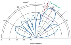
Beamwidth provides a metric of angular resolution for antennas. Most commonly, beamwidth is defined by either the half-power beamwidth (HPBW) or the null-to-null spacing of the main lobe (FNBW). To find the HPBW, we move 3 dB down from the peak and measure the angular distance (Fig. 1).
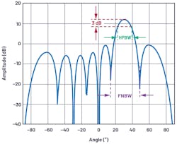

Then solving for ∆Φ gives 0.35 rad. Use Equation 2 and solve for θ:

That θ is the peak to 3 dB point, which is half of our HPBW. Therefore, we simply double it to arrive at the angular distance between the 3-dB points. This results in an HPBW of 12.8º.
We could repeat this for an array factor equal to 0 and obtain the first null-to-null spacing angle of FNBW = 28.5º, for the previously mentioned conditions.
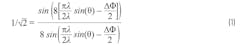
For uniform linear arrays, an approximation for HPBW1,2 is given as Equation 3:

Figure 2 plots beamwidth vs. beam angle for several element counts in the condition of a λ/2 element spacing. From this graph, it’s worth noting some observations relative to array sizes under development in the industry.
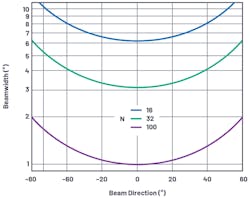
A 1° beam accuracy requires 100 elements. If this is desired in both azimuth and elevation, it results in a 10,000-element array. The 1° accuracy is only at boresight under near-ideal conditions. Maintaining 1° accuracy in a fielded array across a variety of scan angles will further increase the element count. This observation then sets a practical limit for beamwidth with very large arrays.
A 1,000-element array is common in the industry. Thirty-two elements in each direction provides an element count of 1024 and can yield a beam accuracy of less than 4° near boresight.
A 256-element array, which can be mass-produced at low cost, can still have a beam-pointing accuracy less than 10°. This may be perfectly acceptable for many applications.
Also note that for any of these cases, the beamwidth doubles at 60° offsets. This is from the cosθ in the denominator and is due to the foreshortening of the array; that is, the array appears to be a smaller cross-section when viewed from an angle.
Combining Element and Array Factors
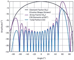
The previous section only considered the array factor. But to find the total antenna gain, we also require the element factor. Figure 3 illustrates an example. In this example, we use a simple cosine shape as the element factor, or normalized element gain, GE(θ). The cosine rolloff is common in phased-array analysis and can be visualized if considering a flat surface. At broadside, there’s a maximum area. As the angle moves away from broadside, the area visible reduces following a cosine function.
The array factor, GA(θ), was used for a 16-element linear array, with a λ/2 spacing, and a uniform radiation pattern. The total pattern is a linear multiplication of the element factor and array factor, so in a dB scale, they can be added together.
A few observations as the beam moves off boresight:
- The main beam loses amplitude at the rate of the element factor.
- The sidelobes on boresight have no amplitude loss.
- The result is the sidelobe performance of the overall array degraded off boresight.
Antenna Plots: Cartesian vs. Polar
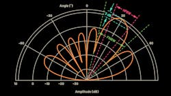
The antenna pattern plots used up to this point have been in cartesian coordinates. However, it’s common to plot antenna patterns in polar coordinates as they’re more representative of energy radiating spatially outwards from the antenna.
Figure 4 is a redrawn version of Figure 1 but using polar coordinates. Note that this is the exact same data, point for point—it’s just redrawn with a polar coordinate system. It’s worthwhile to be able to visualize the antenna pattern in either representation as both are used in literature. For most of this text, we will use cartesian coordinates—in this representation, it can be easier to compare beamwidth and sidelobe performance.
Array Reciprocity
Up until this point, all of the diagrams and text have described a signal that the array is receiving. But how would this change for a transmit array? Fortunately, most antenna arrays are reciprocal. Therefore, all of the diagrams, equations, and terminology are the same for transmit as they are for receive.
Sometimes it’s easier to think of the beam as being received by the array. And sometimes, perhaps in the case of grating lobes, you may find it more intuitive to think of the array as transmitting a beam. In this article, we generally describe the array as receiving a signal. But if this is harder to visualize, then you can equally think of the same concepts on the transmit side.
Summary
This concludes the first segment of this series. We introduced the concept of beamsteering with a phased array. We derived, and showed graphically, the equations to calculate phase shift across the array for beamsteering. Then, we defined array factor and element factor with observations of how the number of elements, the spacing between elements, and the beam angle impacts the antenna response. Finally, we showed a comparison of antenna patterns in cartesian vs. polar coordinates.
Upcoming articles in this series will further explore phased-array antenna patterns and impairments. We’ll study how antenna tapering reduces sidelobes, how grating lobes are formed, and the impact of phase shift vs. time delay in wideband systems. The series will finish with an analysis of the finite resolution of the delay block and how it can create quantization sidelobes and degrade beam resolution.
Authors’ Note: This series of articles is not intended to create antenna design engineers, but rather to help the engineer working on a subsystem or component used in a phased array to visualize how their effort may impact a phased-array antenna pattern.
Peter Delos is Technical Lead and Bob Broughton is Director of Engineering for Analog Devices’ Aerospace and Defense Group; Jon Kraft is Senior Staff Field Applications Engineer at Analog Devices.
References
1. Balanis, Constantine A. Antenna Theory: Analysis and Design. Third edition, Wiley, 2005.
2. Mailloux, Robert J. Phased Array Antenna Handbook. Second edition, Artech House, 2005.
3. O’Donnell, Robert M. “Radar Systems Engineering: Introduction.” IEEE, June 2012. Skolnik, Merrill. Radar Handbook. Third edition, McGraw-Hill, 2008.
>> Microwaves & RF Resources
.. >> Library: Article Series
.. .. >> Topic: Phased-Array Antenna Design
.. ... .. >> Phased-Array Antenna Patterns
About the Author
Peter Delos
Technical Lead, Aerospace and Defense Group, Analog Devices
Peter Delos is a technical lead in the Aerospace and Defense Group at Analog Devices in Greensboro, N.C. He received his BSEE from Virginia Tech in 1990 and MSEE from NJIT in 2004. Peter has over 25 years of industry experience, with most spent designing advanced RF/analog systems at the architecture level, PWB level, and IC level. He’s currently focused on miniaturizing high-performance receiver, waveform generator, and synthesizer designs for phased-array applications.
