11 Myths About Inference Acceleration

This article appeared in Electronic Design and has been published here with permission.
It’s important to understand that an inference accelerator is a completely new kind of chip, with many unknowns for the broader market. In our industry, there’s a learning curve for everything, from how to architect chips to where they belong and how to compare the performance of one approach to another. This has created a lot of misconceptions because vendors and customers don’t know enough about inference acceleration and, in some cases, are releasing misleading data. It’s time to dispel 11 of those most common myths.
1. All inference is in the data center.
Today, the bulk of inference acceleration is in the data center; however, in the future, more inference acceleration will occur outside of the data center at “the edge” (Fig. 1).
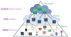
Most high-end cell phones already have some inference acceleration. For example, there are many users of Nvidia Tesla T4 PCIe inference cards in edge servers (enterprises, large stores, bank chains, and so on), and many new inference applications are appearing at the edge. The key to growth of edge inference is solutions that offer data-center-class inference throughput at power levels in the low double-digit watts.
2. Large batch sizes are OK.
The first dedicated inference accelerator was the Google TPU. It used a large systolic array to achieve high throughput, but only for large batch sizes.
In the data center, “pools” of data are waiting to be processed and much of the processing isn’t time-critical. Thus, large batch sizes make sense in such use cases.
However, at the edge, most applications are “streaming.” There’s a sensor, such as a megapixel image sensor, capturing 30 images/s and the images need to be processed as they’re received. To batch them would require storage, which means nothing happens till the Nth image is received. Thus, the latency would be longer.
3. TOPS values predict performance.
Teraoperations/second, or TOPS, is defined as:
(number of MACs on the accelerator) × (the clock frequency) × 2 (1 MAC = 2 Operations)
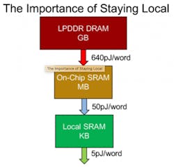
A TOPS value tells you only about the peak possible compute capacity. It tells you nothing about whether the MACs will be efficiently utilized in processing a given neural-network model. Effective inferencing chips are designed to move data through them very quickly, which means very-high-speed data processing and memory transfers.
On any inference accelerator there are:
- MACs
- On-chip SRAM
- Off-chip DRAM
- Control logic
- On-chip interconnects between all units
It’s the number, ratio, and architecture of all these blocks, plus the software that controls them, that will determine actual performance. TOPS (or MACs) is just one piece of the puzzle.
4. ResNet-50 neural-network performance predicts overall performance.
Looking at ResNet-50 neural-network performance is a step in the right direction. It’s a more accurate predictor than simply relying on TOPS values as it exercises all of the elements in an accelerator. Customers new to neural networks assume that if they measure Accelerator A’s frames/s rate on ResNet-50 vs Accelerator B’s ResNet-50 frames/s rate, the resulting relative ratio will hold up for other models, such as the YOLOv3 object-detection algorithm running at 2 Mpixels.
Sadly, this is not the case.
The root problem is that ResNet-50 uses 224 × 224 images, which are very small. Typically, customers want to process 2-Mpixel images, which are >40 times larger. Not only that, but the intermediate activations are even larger, going up to 64 MB. Thus, ResNet-50 doesn’t stress the memory subsystem. The problem is easily solved by running ResNet-50 on 1440 × 1440 images (2 Mpixels), because then the performance will be in ballpark of YOLOv3 for 2-Mpixel images.
5. Any model predicts performance.
Flex Logix has worked with multiple customers using neural networks for a wide range of applications. We’ve seen that the relative performance between two different accelerator architectures can vary by as much as 100X between the most extreme models.
As a result, the only benchmark you should be asking for is how your model runs on any given inference accelerator. If your model is a derivative of something like YOLOv3, then the starting model is a reasonable predictor.
6. Throughput for batch = 1 is the best indicator of performance.
If an accelerator has one “engine,” then throughput for batch = 1 is the inverse of latency. However, if some accelerators (such as Nvidia’s Xavier AGX/NX) have multiple accelerators, they can quote throughput of, say, 50 frames/s, but the latency is not 20 ms/frame because three engines are processing in parallel. In fact, for many models, the latency is quite imbalanced, so only one engine can actually be used for a streaming application processing a single sensor.
This shows that it’s the combination of latency and throughput that matters for most applications.
7. All inference is INT8.
Many customers want to run their models in floating-point mode. There are three reasons behind this thinking:
- The effort to quantize isn’t worth it for their scale of production.
- They don’t want to give up any accuracy.
- They don’t have a dataset for retraining the quantized model.
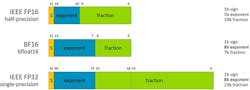
Very high-volume applications will eventually go to an INT8 data model, but many others will not. As Figure 2 shows, customers prefer the BF16 floating-point format because they can convert their FP32 model weights very easily by just rounding off the fraction (the exponent is the same number of bits for BF16 and FP32).
8. MACs and memory predict performance.
The interconnect or network-on-chip (NOC) that connects computation and memory is rarely discussed in articles about inference acceleration. However, it’s the “plumbing,” along with the software, that’s perhaps the most critical part of the architecture for a quality inference accelerator.
We see many inference accelerators with very large numbers of TOPS and huge DRAM bandwidth that don’t deliver much more performance than much smaller accelerators with fewer TOPS and a single DRAM. The reason for that is the interconnect. Most accelerators use traditional processor approaches: buses that connect multiple compute units to pools of memory; and caches of memory. This results in large amounts of bus contention, which leaves the MACs data-starved and poorly utilized.
The best interconnects are deterministic and non-blocking between memory input, MACs, and memory output.
9. Software is the easy part of inference accelerators.
Want to design a world-class inference accelerator? If so, then the software team had better be as large as the hardware team. The software also needs to be developed in parallel with the hardware. In fact, if the software is not ready before silicon, how can the hardware be benchmarked on models to verify performance and power consumption before freezing the chip design?
Software and hardware need to be co-designed for an efficient inference accelerator.
10. Supporting all operators is easy.
Approximately 500 operators are used in integer and floating-point versions of TensorFlow Lite and ONNX, which are popular open-source tools for modeling machine learning. All inference accelerators use optimized hardware to accelerate performance, which means there’s software work involved in supporting each operator.
Many accelerators have been announced with no benchmark or with only one benchmark. This is likely due to the time required to support a wide set of operators. Over time, all vendors will traverse the learning curve, but in the early stages, it’s likely only the most popular operators will be supported in initial releases.
11. Layers must be processed one at a time.
Some accelerators have hardware and software that allow two or more layers to be fused, which has the big benefit of eliminating in some cases very large intermediate activations that would otherwise have to be written to DRAM, stalling processing and burning power (Fig. 3).
Flex Logix’s nnMAX neural network architecture, for example, can fuse layers as shown in Figure 4 so that Layer 0 computes and feeds its intermediate activation directly into Layer 1 computing simultaneously. If not for this, the 64-MB intermediate activation of Layer 0 would need to be stored to DRAM and then read back, burning power and stalling computation.
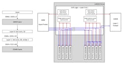
Accelerators that can do this have more flexible architectures that allow compute and memory resources to be connected and programmed in many ways.
Geoff Tate is CEO of Flex Logix Inc.
About the Author
Geoff Tate
CEO and Co-founder, Flex Logix Inc.
Geoff Tate is CEO and co-founder of Flex Logix Inc. Earlier in his career, he was the founding CEO of Rambus. Prior to Rambus, Mr. Tate worked for more than a decade at AMD, where he was Senior VP, Microprocessors and Logic. Prior to joining Flex Logix, Tate ran a solar-energy company and served on several high-tech boards. He currently is a board member of the MRAM company Everspin. Tate holds a Bachelor of Science in Computer Science from the University of Alberta and an MBA from Harvard University. He also completed his MSEE (coursework) at Santa Clara University.
