Phase-Noise Modeling, Simulation, and Propagation in Phase-Locked Loops (Part 1)
What you’ll learn:
- Some brief theory and typical measurements of phase noise.
- Standard analysis of PLL phase noise used by most CAD applications.
- How to produce the lowest phase noise at a PLL output.
- A standard design procedure for a typical Type 2, second-order loop.
Phase-locked loops (PLLs) are ubiquitous in today’s high-tech world. Almost all commercial and military products employ them in their operation, and phase (or PM) noise is a major concern. Frequency (or FM) noise is closely related (instantaneous frequency is the time derivative of phase) and generally considered under the umbrella of phase noise (perhaps both might be considered “angle noise”). Amplitude (or AM) noise is another consideration.
While both affect PLL performance, amplitude noise is usually self-limiting and of no consequence. Phase noise, therefore, at the PLL output and of the RF components, is the dominant concern. Of course, output phase noise is the ultimate concern—it depends critically on the phase noise of each component.
A number of factors contribute to component phase noise, such as power supplies, EMI, and semiconductor anomalies, to name a few. Understanding these factors allows us to implement mitigation strategies for component phase noise and, ultimately, output phase noise.
The kind of PLL we’re discussing is of the analog hardware variety rather than the digital or software variety. The general topology of such a PLL is a single-loop system that contains a precision reference, reference divider, feedback divider, possible prescaler, voltage or current (aka charge pump) phase detector, loop filter, and voltage-controlled oscillator (VCO). These components may all be discrete or some of them may be contained in an IC. In any event, we show how phase noise in general can be analyzed and how RF component phase noise propagates through a PLL to determine its output phase noise.
In Part 1, we discuss some brief theory and typical measurements of phase noise along with the analysis (modeling, simulation, and propagation) thereof, and show in detail the method used by most computer-aided-design (CAD) applications.
Brief Theory and Typical Measurements of Phase Noise
Phase noise is an important and complex subject with ongoing research as well as a tenuous understanding of its origins and a questionable mathematical foundation. However, a number of approximations and workarounds are utilized to produce excellent theoretical and practical results.1,2,3 It’s a mature subject with much literature available. Several instruments are available that accurately measure phase noise, and innumerable fielded systems with PLLs have controlled phase-noise characteristics.
Here, we briefly review the theory of phase noise in the time and frequency domains as well as the transformation between domains for both the baseband (BB) realm (BB noise signal that phase-modulates the RF carrier signal) and the RF realm (RF carrier signal that’s phase-modulated by the BB noise signal).
Also, we summarily review the typical measurements of phase noise for both realms in the frequency domain, which are, of course, different equivalent representations of the same phenomenon and give the same result.
The BB realm is considered the less important realm, but is of interest for the origins of phase noise and offers better measurement accuracy than the RF realm. The RF realm is considered the more important realm and is of interest for the observable manifestations of phase noise, though it has inferior measurement accuracy to the BB realm.1,8 In addition, we investigate the equivalency of both types of measurements.
As is well known in all of physics, there are deterministic and non-deterministic (aka random, stochastic or probabilistic) processes. In PLLs, these processes are signals, which can be expressed in both the time and frequency domains for both realms, with the two domains related through transform theory by the Fourier transform.
To use (in this case, continuous) transform theory, a system is modeled as a (continuous) linear time-invariant network, which means a PLL must be in a locked state. In contrast, the model of a PLL in an unlocked state is nonlinear; thus, transform theory cannot be applied.
Moreover, the transformation between domains is direct for deterministic signals and indirect for random signals. Direct means the transformation is done directly between the time and frequency domains because the direct transform exists. Indirect means that there’s an intermediate step in the transformation between domains, which is to calculate the autocorrelation function of the random signal and take its time-average, and then take the transform, because the direct transform doesn’t exist.6
Phase noise, then, in an RF system or an RF component, is produced when an internal and/or external BB random (noise) signal, of both known and unknown origin, phase-modulates a system's or a component's internal RF deterministic (carrier) signal. It follows, of course, that phase noise, being a random phenomenon or signal, is imbued with an indirect transformation.
Generally, for a random signal in the frequency domain, the spectrum as a voltage spectral density (VSD) doesn’t exist. However, the spectrum does exist as a power spectral density (PSD) having only magnitude and no phase information. In contrast, for a deterministic signal in the frequency domain, the spectrum generally does exist as a VSD, having both magnitude and phase information, which also, of course, has a PSD by extension.
Moreover, in the frequency domain for the BB realm, the spectrum is a low-pass (or quasi-low-pass) function, and for the RF realm the spectrum is a bandpass function. Additionally, in this discussion, we’re working with only positive one-sided (OS) spectra and positive single-sideband (SSB) phase-noise information in contrast to two-sided (TS) spectra and double-sideband (DSB) phase-noise information.
We also note that in the time domain, phase noise is typically referred to as phase jitter and in the frequency domain it’s typically referred to as stated-phase noise. The phenomenon in both domains is related through the definition of instantaneous frequency being the time derivative of phase.1,8,10
With the above background in mind, we briefly review some theory in the time and frequency domains as well as the transformation between domains for the BB realm. In this realm, our theory and analysis basically exist in principle since there’s no analytical expression for our random (noise) signal in the time domain (which is where our analysis begins). Hence, after transformation, there’s no analytical expression in the frequency domain. We have the following mathematical representations and transform steps:6,7,8
1. The time domain function or phase waveform, which is a real (non-complex) random process with a zero-mean Gaussian probability density function, ϕ(t):

where t is the time.
2. The autocorrelation function of (1), Rϕ (t, τ):

where τ is the positive time increment between measurements and Eop{...}is the statistical average operator.
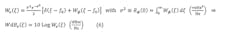
3. The Fourier transform of the time-average of Equation 2, giving the unnormalized (UN) BB frequency domain function or PSD, Wϕ(ξ) or WdBϕ(ξ):

where ξ is the frequency, Aop{...}is the time average operator, and Fop{...} is the Fourier transform operator. Typical plots of the phase waveform and its UN BB PSD are shown in Figure 1a and 1b.
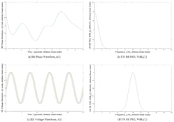
1. Typical plots in phase-noise theory of (a) the baseband (BB) phase waveform, ϕ(t), (b) the unnormalized (UN) BB power spectral density (PSD), Wdbϕ(ξ), (c) the RF voltage waveform, v(t), and (d) the UN RF PSD, Wdbv(ξ).
Next, we briefly review similar theory in the time and frequency domains as well as the transformation between domains for the RF realm. In this realm, our theory and analysis are fairly analytical since there’s a fairly analytical expression for our deterministic (carrier) signal in the time domain (which, once again, is where our analysis begins). Hence, after transformation, there’s a fairly analytical expression in the frequency domain.
For a “reasonable” phase waveform deviation (aka small angle..., small modulation index..., or narrowband PM...approximation) of ≤ 0.2 rad (≤ 11.5°), where a PM spectrum is basically identical to a DSB AM spectrum—which is the case for all practical phase noise issues—we have the following mathematical representations and transform steps (details not shown for brevity):7,8,10
4. The time domain function or voltage waveform (also a function of the BB parameters), v(t):

where V is the statistical mean amplitude, f0 is the carrier frequency, and Θ is the initial phase (V is a special case of the general amplitude, V + a(t), where a(t) is the statistical zero-mean amplitude noise with a(t) = 0, since, as mentioned, it’s self-limiting and of no consequence):
5. The autocorrelation function of Equation 4 (again also a function of the BB parameters), Rv(τ):

where Rϕ(0) is Rϕ(τ) with τ = 0, which is the variance of ϕ(t).
6. The Fourier transform of the time average of Equation 4 (once again also a function of the BB parameters) giving the UN RF frequency domain function or PSD, Wv(ξ) or WdBv(ξ):
where d(ξ – f0) is the Dirac delta or unit impulse function and Wϕ(ξ – f0) is the UN BB PSD, Wϕ(ξ), translated from the BB realm to the RF realm through the modulation process. Typical plots of the voltage waveform and its UN RF PSD are shown in Figure 1c and 1d.
It should be noted that if ϕ(t) is strict-sense stationary (a reasonable assumption), it may be proved that v(t) is at least wide-sense stationary. In this case, the Weiner-Khinchin theorem holds, with Rϕ(t, τ) and Rv(t, τ) becoming functions only of τ, [Rϕ(t, τ) → Rϕ(τ) and Rv(t, τ) → Rv(τ)] and therefore finding the time-averages of Rϕ(τ) and Rv(τ) aren’t necessary. Hence, Wϕ(ξ) and Wv(ξ) are the Fourier transforms of Rϕ(τ) and Rv(τ) themselves.1,6,7,9
Then, with the above brief theory in mind, we summarily review the typical measurements of phase noise for both the BB and RF realms in the frequency domain.
Measurement in the BB Realm
In the UN BB PSD above, a particular frequency is selected and its power in a 1-Hz bandwidth is divided by the total integrated power over the low-pass spectrum, which gives the normalized (NM) BB PSD, Lϕ(ξ) or LdBϕ(ξ):

where ξ is the particular frequency, Pz is the total integrated low-pass power, and dBz is decibels relative to Pz. The measurement is indirect, using a signal source analyzer, which demodulates, measures, processes, and displays the BB signal to produce Lϕ(ξ) or LdBϕ(ξ) [Wϕ(ξ) contains DSB information and therefore the factor of 2 is needed in the calculation of Lϕ(ξ) to give SSB information]. It’s considered more accurate than that done in the RF realm.1,8
Measurement in the RF Realm
In the UN RF PSD above, a particular offset frequency from the carrier is selected. Its power in a 1-Hz bandwidth is divided by the total integrated power over the bandpass spectrum, which gives the NM RF PSD, Lv(f) or LdBv(f):

where f is the particular offset frequency from the carrier (f = ξ − f0 with ξ ≥ f0), Pc is the total integrated bandpass power, and dBc is decibels relative to Pc. The measurement is direct, using a spectrum analyzer with phase-noise processing capability, which measures, processes, and displays the RF signal to produce Lv(f) or LdBv(f). It’s considered less accurate than that done in the BB realm.1,8
Equivalency of Both Measurements
As mentioned, Lϕ(ξ) or LdBϕ(ξ) and Lv(f) or LdBv(f) are different representations of the same phenomenon and logically should give the same result for all practical phase-noise issues (where, also as mentioned, the phase deviation is considered “reasonable”). Therefore, for this case, they’re equivalent and do give the same result, which is termed the NM PSD, L(f) or LdB(f). The BB and RF realm subscripts (ϕ and v) are dropped and no subscripts are used (even the “reasonable” condition has some anomalies where approximations with academic and practical arguments must be used):1,10

where the typical display has f as the offset frequency from the carrier for the x-axis in units of Hz on a logarithmic scale and LdB(f) as the NM RF PSD for the y-axis in units of dBc/Hz on a linear scale, for both the indirect and direct measurements mentioned above, to ultimately relate everything to the RF realm (Fig. 2).
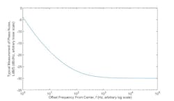
2. Typical measurement of phase noise for both the baseband and RF realms in the frequency domain.
It should be noted that if the “reasonable” condition isn’t met, then Bessel function mathematics must be used to relate Lϕ(ξ) to Lv(f). Therefore, both measurements would not be equivalent, would give different results, and would be considered a catastrophic problem.
Analysis (Modeling, Simulation, and Propagation) of Phase Noise=
Armed with the above information, we now come to the analysis of phase noise in a PLL and how it’s modeled and simulated in general. Also discussed is how RF component phase noise is propagated through the PLL to determine its output phase noise. Typically, phase noise is effectively modeled using the “General Phase Noise Model” (Fig. 3) with its standard integer power series:

3. General Phase Noise Model used in the analysis (modeling, simulation, and propagation) of phase noise.
where h is a weighting coefficient and f is the offset frequency from the carrier.1,7 It’s then simulated with any standard application (in this case, we use MATLAB). Finally, propagation of component phase noise through the PLL to determine its output phase noise is done using the General PLL Block “Diagram & Phase Noise Propagation Model” (Fig. 4).
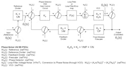
4. General PLL block diagram and Phase Noise Propagation Model used in the analysis (modeling, simulation, and propagation) of phase noise.
Furthermore, to simplify the analysis, all components’ phase noise is approximated as being uncorrelated (a reasonable assumption) so that their NM PSDs add directly, rather than having to deal with correlated signals, which significantly complicates the analysis. Analysis is then done with the following Phase Noise Analysis Procedure:4,5
1. The PLL must be represented as a (in this case continuous) linear, time-invariant network, which means it must be locked at one of its outputs.
2. All components’ phase noise must be approximated as being uncorrelated.
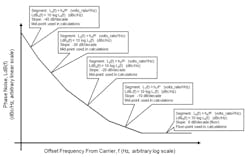
3. Each component’s phase-noise plot is obtained from its datasheet and the “General Phase Noise Model” (Fig. 3) is fit to each component's plot to determine the segments of the general model (some of which may not exist) that match each component's plot.
4. For each component's fitted General Phase Noise Model, one phase noise point, LdBj(fk) (j,k = 0,a; 1,b; 2,c; 3,d; 4,e), within each segment is obtained for use in calculations (the mid-point within a segment is often used). Convert all log values to linear values, LdBj(fk) ÞLj(fk):
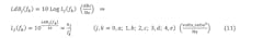
5. Each component’s fitted General Phase Noise Model coefficients, hj, are calculated using the phase-noise points from step 4 (some of which may be zero):

6. Each component’s fitted General Phase Noise Model coefficients, hj, from step 5 are used to form each component’s phase-noise model, Lci(f):

which can be simulated to produce component phase noise curves.
7. Each component’s phase-noise model, Lci(f), from step 6 is multiplied by its applicable transfer function (output or error; to be discussed later) magnitude-squared, |T(f)|2, to get its propagated phase noise model, Lco(f):

which can be simulated to produce component propagated phase-noise curves.
8. Each component's propagated phase noise model, Lco(f), from step 7 is summed together with all others to get the output phase noise model, Lto(f):

which can be simulated to produce the output phase noise curve.
This, then, is our phase-noise analysis (modeling, simulation, and propagation) procedure. As mentioned, it’s the method used by most CAD applications for phase-noise analysis.
The above information will be used in the upcoming Part 2, where we design a hypothetical PLL frequency synthesizer as an example to be used for analysis.
References
1. F.M. Gardner, "Phaselock Techniques", 3rd ed., John Wiley, Hoboken, NJ, 2005.
2. R.E. Best, "Phase-Locked Loops, Design, Simulation and Applications", 6th ed., McGraw-Hill, New York, NY, 2007.
3. P.V. Brennan, "Phase-Locked Loops: Principles and Practice", McGraw-Hill, New York, NY, 1996.
4. E. Drucker, "Phase Lock Loops and Frequency Synthesis for Wireless Engineers", 1997, Frequency Synthesis & Phase-Locked Loop Design, 3 Day Short Course, Besser Associates, Mountain View, Calif., 1999.
5. F.C. Weist, "Phase Locked Loop Basics for Frequency Synthesizer Applications", Short Course, Clarksburg, Md., 2011.
6. P.Z. Peebles, Jr., "Probability, Random Variables and Random Signal Principles"', McGraw-Hill, New York, NY, 1980.
7. A. Godone, S. Micalizio, and F. Levi, "RF spectrum of a carrier with a random phase modulation of arbitrary slope", Istituto Nazionale di Ricerca Metrologic, INRIM, Strada delle Cacce 91, 10135 Torino, Italy, Metrologia, vol. 45, pp. 313-324, BIPM and IOP Publishing Ltd., Bristol BS1 6HG, UK, May 2008.
8. B. Nelson, "Phase noise 101: basics, applications and measurements", Keysight Technologies, 2018.
9. A. El Gamal, EE278 Lecture Notes 7: "Stationary random processes", Dept. of Electrical Engineering, College of Engineering, Stanford University, Stanford, CA, Autumn 2015.
10. K. J. Button, ed., Infrared and Millimeter Waves, Volume 11: Millimeter Components and Techniques, Part III, Chapter 7: "Phase Noise and AM Noise Measurements in the Frequency Domain", A. L. Lance, W. D. Seal and F. Labaar, TRW Operations and Support Group, One Space Park, Redondo Beach, CA, Academic Press, Cambridge, MA, 1984.
About the Author
Frederick Weist
Principal, FCW Sciences
Frederick Weist presently resides in Point of Rocks, Md. He was born in Phila., Pa., on March 25, 1959. He obtained his BS in physics from Drexel University in 1983 and his MS in physics from the same institution in 1992.
Mr. Weist is presently retired, but continues his interest in research and writing by working as Principal at FCW Sciences. His last position was as Principal Engineer/SME with Boeing Co. - Digital Receiver Technology Subsidiary, Germantown, Md. Previously he held positions as Senior Design Engineer with Kratos Defense and Security Solutions - Herley-CTI Division; Principal Engineer with DRS Technologies - Signal Solutions Division; Senior Engineer with Aydin Corp. - Telemetry Division; and Electronics Engineer with the U.S. Naval Air Warfare Center - Aircraft Division (NAWCAD).
His previous interests included research, design and development of systems from dc to 42 GHz, specializing in PLLs, frequency synthesizers, transceivers, subsystems, and components. He’s also worked in the fields of photonics, magnetics, superconductivity, sensors, and servo systems. Present interests include the same as well as integrated microwave/photonics, quantum, and biophysics systems.
Mr. Weist is a member of the American Physical Society and the Institute of Electrical and Electronics Engineers.
