Noise Can Tell Much About Material
Download this article in PDF format.
Noise can hide details, but it can also reveal them. If properly used, noise will tell a great deal about a device under test (DUT), including when a DUT is raw material. For example, the Microwave Noise Field (MNF) test method has the capability to test different objects that can move, as well as objects with granular or irregular composition. When properly applied, the MNF method can provide precise analysis of different types of materials to help optimize the use of those materials in industrial applications.
The MNF method, also known as active radiometry, is a means of using noise rather than continuous-wave (CW) test signals when measuring the insertion loss of different materials.1-3 The DUT or material to be tested is placed between a noise source and a radiometer antenna. The noise field is random with low coherence so that interference effects are negligible close to the radiators.
In addition, a DUT can move within the noise field without invalidating the measurements. A DUT being characterized in the noise field of the MNF method might even be considered as an object surrounded by white light, with little or no effects on the object from the white light.4
For measurements using the MNF method, the power level of the radiated noise in the noise field is very low, with noise measurements typically at nanowatt (nW) levels. A microwave radiometer is required as a detector to determine such low noise levels. The use of wideband noise for device or material testing has certain advantages over the use of measurements performed with CW test signals. In contrast to the MNF method, measurements performed with CW test signals require that a DUT be located in the far-field zone of the test signals, and that the DUT not move at all during testing.
Low-cost radiometers have been designed with the same low-noise block downconverters (LNBs) often found in satellite television receivers. Such LNBs are stable enough for measurement purposes, with good low-noise characteristics. In addition, the C- and Ku-band frequencies used for satellite television reception are internationally protected and managed communications frequency bands, preventing the generation of man-made signals (other than satellite-television signals) within those frequency bands.
Test Setup and Performanc
Fig. 1 shows a typical test arrangement for measuring the insertion loss of a DUT placed between a noise radiator and a radiometer antenna. Any propagation loss due to the short distance between the noise radiator and the antenna must be included in the loss measurements. The typical maximum amount of loss that can be measured with such a setup is 40 to 50 dB. Therefore, the test setup can be mounted on a laboratory bench, and the distance between the noise radiometer and the antenna is preferably less than 30 cm (1 ft.) when using Ku-band components.
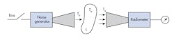
1. The block diagram shows the functions of a basic radiometer to determine the EM loss of an object.
A typical microwave noise radiator (MNR) with an avalanche-diode noise source is characterized by an excess noise ratio (ENR) of 30 dB. The ENR (Eq. 1, in degrees Kelvin) quantifies the noise produced at the output of a DUT by its noise temperature (Tx) above the ambient temperature (To) of the test setup:
Tx = ENR × To (1)
An ENR of 30 dB means that for a typical To of 300 K, the Tx is 300,000 K.
The noise power, Pn, (in W) can be found from Eq. 2:
Pn = kTxB (2)
where k is Boltzmann’s constant (1.38 × 10⁻²³ J/K); B is the noise bandwidth of the system (in Hz), and Tx is the noise temperature (for this case 3 × 10⁵ K). A typical dipole or waveguide-horn noise radiator has a noise bandwidth of several gigahertz, but radiometers with satellite LNBs typically have noise bandwidths of 1.0 to 1.5 GHz or 109 Hz. Using Eq. 2, it is possible to estimate the radiated noise power for such a radiometer:
Pn = kTxB
= 1.38 × 10⁻²³(3 × 10⁵)109
= 4 × 10⁻⁹ W or 4 nW
Fig. 2 presents the range of DUT loss (in dB) that can be measured with a noise radiator with ENRs of 15 and 30 dB, and a radiometer with various temperature resolutions.
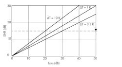
2. The curves demonstrate the measurable loss in a system such as that represented in Fig. 1.
Typical microwave radiometers with satellite LNBs consist of the LNB, an intermediate-frequency (IF) amplifier, and an IF detector (Fig. 3). With an RF bandwidth of 1.0 to 1.5 GHz and noise figure of 1 to 2 dB, the temperature resolution1 can be found from Eq. 3:
dT = Tsn/(Bτ)0.5 (3)
where dT is the minimum detectable temperature step (in degrees K); Tsn is the radiometer noise temperature (including the antenna noise temperature if pointed off target);
B is the predetection bandwidth; and τ is the post-detector smoothing time constant (in seconds). For the frequencies and values mentioned previously, the Tsn is around 350 to 400 K (the radiometer antenna typically sees an ambient temperature wall if the noise radiator is off); B = 1 GHz; and τ can be set to 1 s.
By plugging values into Eq. 3, it becomes
dT = 400/[(10 × e9)(1)]0.5 = 0.12 K
Since simple radiometers are not completely temperature stable, a value of 0.5 to 1.0 K can be used for the value of dT to account for the instabilities.
To improve system resolution and stability, keying is performed with the noise radiator output, and the corresponding ac component for a particular keyed noise input. Fig. 3 shows a noise-detection system that makes use of noise keying. An audio noise keying frequency, such as 1 kHz, can be used as the keying signal. For the MNF test setup, a sound level meter was connected to the radiometer output, to indicate the loss in dB for the noise keying signals.
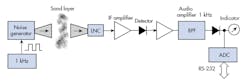
3. This block diagram represents a system that can measure the loss of a moving object by using noise.
With the use of keying, the loss measurement range exceeded 40 dB. The test system response was also tested with a calibrated waveguide attenuator connected between the noise source and the horn antenna to confirm system “linearity” for levels above 40 dB.
Fig. 3 shows the schematic diagram of a practical noise-field measurement system that has been used to measure moisture in sand and to detect flaws in wooden planks, in plywood, in rubber-tire sidewalls, as well as to identify wet spots in paper and fabrics. Fig. 4 plots a comparison of measurements of moisture-based loss in sand, using CW test signals and noise field data.
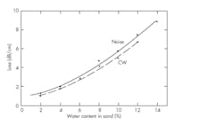
4. Loss in sand increases as a function of water content, shown for a wavelength of about 3 cm.
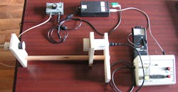
The plots showing the influence of increased moisture on increased loss are quite similar. However, using a CW test signal at 10 GHz (at a wavelength, λ, of 3 cm) is not practical, since the sand layer must be fixed and cannot move to allow the use of a CW test signal. Using a noise field for such measurements is greatly preferred since the measurement data are not impacted by any movement of the sample material under test. Fig. 5 shows a photograph of the experimental MNF test setup, with keying circuit for the noise radiator, the radiometer, its analog indicator, and the logarithmic sound-level meter.
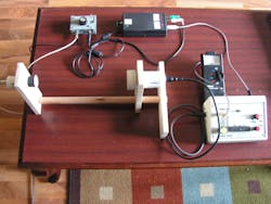
5. This experimental setup includes a keying circuit for the noise radiator, the radiometer, its analog indicator, and the logarithmic sound-level meter.
Useful Applications
The first application of the MNF method was described in ref. 2 for the measurement of loss due to the moisture content of sand. Figure 4 shows a calibration curve for conventional CW test signals and for noise-based measurements on sand moisture levels from 0 to 14% (sand cannot be moister than this).
The industrial MNF system performed measurements on sand moving on a conveyor belt. A sand layer approximately 3 cm thick was maintained with a steel ruler on the rubber conveyor belt. Some loss, about 4 dB, in the system was discounted to account for measurement variations. However, sand movement within the system did not affect the measurement of the sand-moisture value, providing that some integration was performed for smoothing.
In this measurement system, noise keying at 1 kHz was used, with antennas set 15 cm apart. The Ku-band system, named Scout-1, has been used in several concrete-mixing plants since 1990 as a means of measuring moisture content of moving materials. A similar system was designed for use at C-band frequencies to measure the moisture content of wood chips and wooden planks in a wood-drying plant and in an incinerator.
In 2014, the Czech Technical University, Institute of Materials, sought a method to detect flaws in the sidewalls of rubber tires for a rubber tire manufacturer. The manufacturer used a sidewall-looking camera to detect sidewall thickening or thinning. Samples with marked flaws were tested in the setup shown in Fig. 5, at Ku-band frequencies, to confirm the known flaws as well as to identify whether additional, unseen flaws were present. The rubber tire company then declined to cooperate. Apparently, the MNF system detected more flaws than the rubber tire manufacturer expected to be found. For noise measurements performed on the rubber sidewalls, typical loss was 10 dB on average, with flaws increasing the loss by 3 to 5 dB.
The test setup shown in Fig. 5 was also used to measure the moisture content of wood planks with 1 in. thickness. Cracks and knots in the planks were readily indicated with the MNF method. Also, fiber orientation and moisture were detected by moving planks or plywood by hand between the antennas. The typical loss measured for a dry plank was 10 dB. Flaws and moist spots added 3 to 5 dB to the loss measurements, while knots and cracks in the wood reduced the loss measurements by as much as 3 dB.
Other researchers have used the MNF method to test granular and irregular-shaped materials. In addition to Ku- and C-band frequencies, they have performed wideband sweeps from 1 to 10 GHz as well as measurements around 94 GHz.5
Most LNBs are designed to receive one polarization. But some can receive two orthogonally polarized signals by electrically switching signal polarization with a voltage of 13 or 15 V dc. A linearly polarized signal can be used to distinguish between fibrous materials such as wood or plywood, and a polarization difference can indicate flaws and irregularities in tested samples.
In contrast to attempting to detect weak signal changes (in polarization) in the presence of a strong primary test signal when detecting the results of Mie forward-scatter during material measurements, the MNF test setup was used to identify changes in polarization during testing (i.e., changes in the shapes of the materials being measured). The MNF system was able to easily identify several round objects used to create the Mie forward scatter conditions, including metal rods and plastic rods and tubes.
Metal objects exhibited the greatest on-axis loss, while dielectric materials exhibited two symmetrical peaks with maximum on-axis loss. Most objects measured by the dual-polarization MNF system caused off-axis peaks in the field intensity, as expected according to Mie forward-scattering field theory.
Since the discovery of the MNF method, a number of applications have been evaluated for the technique much like those described here. Basic features have been presented in ref. 1, although not a great deal of feedback resulted in response. The use of the MNF method for industrial material testing features the benefit of the technique’s simplicity and the capability of moving the material or DUT during testing, which is not possible when testing with microwave CW signals. The test approach can gauge loss of more than 40 dB for a material of interest while using extremely low-noise test power levels, leading to the possibility of using the MNF method for analysis in medicine and biology as well as for material research.
References
1. Jiri Polivka, “Noise Can Be Good, Too,” Microwave Journal, March 2004, pp.66-78.
2. Jiri Polivka, “Microwave Radiometry in Measuring Sand Moisture,” 3rd International Workshop on Electromagnetic Wave Interaction with Water and Moist Substances, Athens, GA, April 11-13, 1999.
3. Jiri Polivka, “An Overview of Microwave Sensor Technology,” High Frequency Electronics, April 2007, pp. 32-42.
4. Jiri Polivka, P. Fiala, and J. Machač, “Microwave Noise Field Behaves Like White Light,” Progress in Electromagnetic Research, Vol. 111, 2011, pp. 311-330.
5. B. Kapilevich and B. Litvak, “Noise Versus Coherency in MM-Wave and Microwave Scattering from Inhomogeneous Materials,” Progress in Electromagnetic Research B, Vol. 28, 2011, pp. 35-54.
6. “Scout-1” sand-moisture measuring system; more details available at www.ok1icz.cz.

