VNA Applications in the Quantum-Computing Hardware Stack

What you'll learn:

• What is a qubit?
• What frequencies are used for superconducting qubits?
• How is a VNA employed to evaluate the qubit?
• How does a qubit work?
• Managing SNR and thermal noise in qubit output signals.
• Industry challenges with quantum computing.

In the future, quantum computing will solve many significant problems, with some of the most exciting applications coming in the field of medicine. The function of a protein is determined by how it folds, and the folding mechanics are extremely complicated to solve with conventional computers. However, it’s easily handled with a quantum computer. This will lead to a greater understanding of human biology. Faster and better chemical simulations will lead to new drugs to treat disease. 

We’ll see quantum computers used in fusion research, logistics and supply-chain optimization, climate modeling, and materials measurement, too. But creating a quantum computer with thousands of qubits and suitable error correction is probably several decades away. It’ll take many years of research to optimize designs and scale up into large systems.

The vector network analyzer (VNA) is a formidable instrument for quantum-computer engineering and research. Quantum computing depends on the RF resonance of the qubit and one or more external resonators coupled to it. RF signals must be delivered to and read back from these external resonators. The resonant frequencies and coupling between resonators and the Josephson junction have to meet specific requirements and must be measured. Intentional coupling between qubits may also be implemented to allow for entanglement. 

Qubits and the low-noise parametric amplifiers that follow them operate at very low signal levels. With these low signal levels, cable loss must be characterized to ensure the delivery of accurate signal amplitudes and produce an acceptable signal-to-noise ratio. All of these criteria require a VNA for design verification.

In this introduction, we’ll examine a typical superconducting qubit system. Ion-trap designs aren’t considered here, as the measurement requirements are quite different.

What is a Qubit?

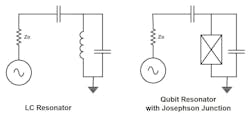
A qubit is an anharmonic resonator. A simple LC harmonic resonator (Figure 1, left side) resonates at a fundamental frequency, Fr, but also at the harmonics of that frequency: 2Fr, 3Fr, and so on.

In the quantum world, frequencies are related to energy levels so that:

E = hf Joules,

where E is the energy, h is Planck’s constant, and f is the frequency.

Each frequency of a harmonic oscillator represents an energy state, and the transition from one state to the next is given by hf, as shown in the diagram on the left side of Figure 2. If a qubit were made with a harmonic resonator, it would be impossible to control its energy state. Application of energy hf could drive the qubit from the ground state, (|0>) to the first excited state, (|1>) or from the first excited state to the one above it, or the one above that. This is undesirable.

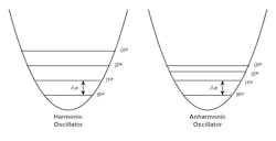
A qubit utilizes an anharmonic resonator with a Josephson junction¹ replacing the inductor, as shown on the right side of Figure 1. The result is the unevenly spaced energy levels shown on the right side of Figure 2.

A Josephson junction has the useful nonlinear property of its inductance varying with the energy of the resonance where the inductance follows the formula:

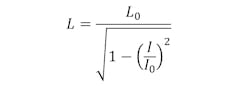
Here, L₀ is a characteristic inductance, I is the applied current, and I₀ is a critical cutoff current. The inductance is very nonlinear, particularly for currents close to I₀. This peculiarity causes the uneven potential energy levels. Because of the uneven bandgap energy spacing, an input energy of △e to the qubit causes a transition from the ground state to the first excited state, and no other transition is possible.

Atoms also have this distinctive uneven energy separation, so a qubit has been called an “artificial atom.”¹ The ion-trap type of quantum computer uses this property directly. The superconducting Josephson junction qubit most often used in research due to its simplicity of manufacture is the Transmon qubit, first introduced by Koch, et al, and studied extensively at Yale University.²

What Frequencies are Used for Superconducting Qubits?

The frequencies used in Josephson junction qubit resonators and filters range from 2 to 10 GHz. These high frequencies are required to ensure that resonator energy levels are many times higher than the thermal energy at the 10- to 20-mK temperatures at the bottom of the cryostat.

Thermal energy is given by kT, where k is Boltzmann’s constant and T is the Kelvin temperature. Electromagnetic (EM) photon energy is given by hf, where h is Planck’s constant, and f is the EM frequency in hertz. We want hf >> kT. At 15 mK, the thermal energy is equivalent to an EM photon at 312 MHz, so anything over 3 GHz is sufficiently energetic.

This is also why quantum computing must be performed at cryogenic temperatures. Experiments at room temperature would require extremely energetic EM photons at hundreds of gigahertz, making qubit design impractical.

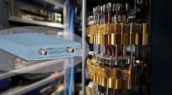
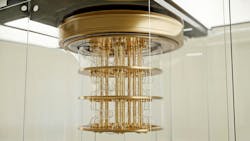
To reach these low temperatures, the quantum computer is housed in a cryostat (Fig. 3), which creates a 10- to 20-mK thermal environment. The temperature is reduced in discrete stages within the cryostat, employing different cooling methods in each stage. With an ambient temperature of 300 K, the internal stages might be at temperatures of 50 K, 4 K, 900 mK, 200 mK, and finally 10 mK.

How is a VNA Employed to Evaluate the Qubit?

A VNA can sweep through the qubit's uneven resonance frequencies and measure them directly. This is critical for determining the energy difference between the ground and first excited states. Such a measurement is required because variation in the qubit's manufacturing process results in some resonant frequency variation. Subsequent operation of the qubit will be done with shaped pulses at the frequencies determined by these measurements.

A VNA reflection measurement (S₁₁) of the qubit will exhibit a dip in the response at the resonant frequency, and resonator Q may be determined from this reflection measurement.³

The coupling—determined by the horizontal capacitor in Figure 1—to the resonant structure impacts the oscillator's Q, which, in turn, affects the duration of time the qubit will remain in its excited state. Low Q, or excessive resonator loading, reduces the relaxation time, designated T1, where the quantum state spontaneously falls back to its ground state as energy leaks away through the coupling capacitor.

In practice, the intrinsic Q of the qubit might be on the order of 1x10⁶, and the Q of the drive coupling about 40X that; thus, the total Q is determined mainly by the qubit structure itself. The coupling's low impact on Q is accomplished by adding readout and Purcell filter resonators, as described below.

How Does a Qubit Work?

The qubit circuit on the right-hand side of Figure 1 is over-simplified. We need the small coupling capacitor (Cq) to prevent loading of the qubit, but it also limits the rate at which energy can be pumped into the system. In fact, the time needed for input and the decay time (T1) would be about equal, meaning the quantum state would likely collapse during measurement.

We provide additional isolation to the qubit by adding a readout resonator at an offset frequency, usually higher by many gigahertz (Fig. 4). Here, the qubit no longer sees the dissipative signal source impedance Zo, instead it sees the short circuit of the readout resonator.

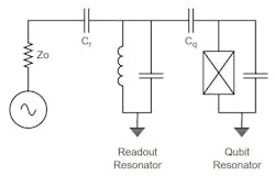
When the qubit moves between its two states, the tiny coupling between the two causes a tiny dispersive shift in the resonant frequency of the readout resonator. Thus, instead of observing the qubit directly, the phase of the readout resonator may be measured.

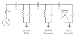
This isolation works so well that it’s repeated, adding another resonator at another offset frequency (Fig. 5). This resonator is called the Purcell filter and multiplies the effect of the readout resonator by about 100, allowing for much longer T1 and enabling readout long before decay occurs.

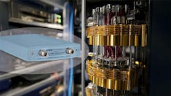
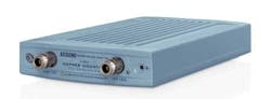
The qubit is a one-port structure where the input is also the output. It’s essential to measure the properties of these resonators with a highly accurate, metrology-grade vector network analyzer like Copper Mountain Technologies’ SC5065 6.5-GHz VNA or SC5090 9-GHz VNA (Fig. 6). These highly precise and compact analyzers, with their small size and low power requirements, are well-suited for the cryo-lab.

The included advanced analysis features of the VNA software can be helpful in the qubit design process. With an external Gaussian pulse modulator on Port 1, frequency offset mode might be used on Port 2 to observe the phase shift of the readout resonator.

Managing SNR and Thermal Noise in Qubit Output Signals

The output signal from the qubit must be amplified with a very low noise amplifier. The signal is perhaps −120 to −130 dBm, and the signal-to-noise ratio (SNR) is critical to prevent read-out errors and create a fault-tolerant computational system. A Josephson junction parametric amplifier⁴ provides about 20 dB of gain and sets the noise figure for the receiver system. Its peculiar design produces high gains at high frequencies with a noise figure approaching the quantum minimum limit.

The parametric amplifier requires one or more “pump” signals higher than the amplified frequency. The amplitude of these signals affects the gain and must be carefully adjusted. Parametric amplifiers are single-port devices, requiring a circulator to separate input from output signals. They’re typically narrowband devices and must be tuned to the frequency of operation. In addition, they exhibit very low input P1dB saturation, on the order of −125 dBm. These characteristics make the system design challenging.

More traditional high electron-mobility transistor (HEMT) amplifiers provide additional gain after the parametric amplifier. These run relatively warm and are in higher temperature zones of the cryostat so as not to overwhelm the cooling capability of the bottom section. A simplified diagram is shown in Figure 7.

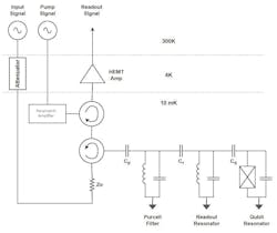
RF attenuators in several cryostat sections reduce the input-signal amplitudes to the tiny levels required to operate the qubit.

Industry Challenges

Every qubit in a quantum computer will likely operate at a slightly different frequency, with readout and Purcell filters also tuned to unique frequencies. Conveniently, this frequency multiplexing allows for simultaneous excitation and readout on a common bus structure.

Unfortunately, the many signals, including the pumping signals to the parametric amplifiers, must be generated by signal synthesizers and modulated to excite the qubits in expected ways. Several thousand sources might be needed for a thousand qubits, with several thousand cables traversing the cryostat from top to bottom. Also, many qubits will be dedicated to error correction and not directly involved in computing. The scalability issue is daunting, and clever solutions will be needed to surmount them.

Perhaps a way can be found to miniaturize the microwave sources and place them within the cryostat. Small-diameter RF cables with lower loss would be helpful. Low-power/low-heat amplifiers to replace the second-stage HEMT amplifiers would also be advantageous. Some decades of work are ahead to sort out these issues.

Quantifying the gains and losses is crucial for all pieces of a quantum-computer system. The amplitude of the input signal to the qubit must be precisely known so that the signal energy causes desired state changes. A rack-mounted microwave source and modulator outside the cryostat develop the input and pump signals, feeding cables that connect to the cryostat. Inside the cryostat, cables proceed through the temperature zones and attenuation stages before finally connecting to the qubit isolator.

The quantum computer might contain hundreds of qubits, so managing the RF system is complicated. One requires a reliable and accurate VNA to measure these cables, attenuators, and isolators. On that front, Copper Mountain Technologies’ VNAs meet these requirements. They’re produced in the United States, and provide measurements traceable to the National Institute of Standards and Technology (NIST).

References

1. J. M. Martinis, M. H. Devoret, and J. Clarke. “Quantum Josephson junction circuits and the dawn of artificial atoms,” Nature Physics, 16:234{237, 2020.

2. J. Koch, T. M. Yu, J. Gambetta, A. A. Houck, D. I. Schuster, J. Majer, A. Blais, M. H. Devoret, S. M. Girvin, and R. J. Schoelkopf. “Charge-insensitive qubit design derived from the cooper pair box,” Phys. Rev. A, 76:42319, 2013.

3. Walker, B. (2020, May 29). “Determining Resonator Q Factor from Return-Loss Measurement Alone,” Microwaves & RF.

4. Lanes, Olivia (2020) “Harnessing Unconventional and Multiple Parametric Couplings for Superconducting Quantum Information.” Doctoral Dissertation, University of Pittsburgh.    (Unpublished)