Algorithms to Antenna: Evaluating Radar Target Detectability
What you'll learn:
- What is a radar's detectability factor?
- Using watefall and stoplight charts to observe results of tests after making design tradeoffs.
- Determining SNR and detectability factor.
In a previous blog, we discussed planning the location of radar sites, focusing on how the signal-to-noise ratio (SNR) of a radar can be used to determine coverage over terrain. The SNR that a radar achieves for a specific area of coverage determines whether a target is detectable.
With the increase in lower cross-section targets such as drones and UAVs, a lot of work is being done in industry and academia to evaluate whether new radar systems are needed to detect small targets or whether existing systems can be upgraded. This work is best started at the analytical level to get early insights into what’s feasible.
We will explore other factors that influence SNR beyond the terrain analysis and then connect back to a scene with mountainous terrain. Once a design is vetted this way, higher-fidelity models can be built at the probabilistic and physics levels, which will be covered in future blogs.
A radar’s detectability factor is defined as a threshold SNR required to make a detection for a specific probability of detection (Pd) and false alarm (Pfa). The maximum range of the system can be estimated as the range at which the available SNR is equal to the detectability factor for a given Pd and Pfa.
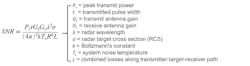
We start with the radar equation, which combines the main parameters of a radar system and allows you to compute a maximum detection range, a required peak transmit power, or a maximum available SNR for a radar system. The radar equation is typically a family of three relatively simple formulas, each corresponding to one of these key performance characteristics. We will use a common form of the radar equation to compute the maximum available SNR at a range R (Fig. 1).
Target range and RCS aren’t under the control of radar designers, but these are the parameters that drive the design change in our example. When the target size is smaller, as is the case with a drone, the SNR available at the receiver must be increased in other ways, such as increasing transmit power, increasing the antenna size, using lower frequency, or increasing the sensitivity of the receiver.
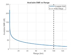
Let’s consider an S-band airport surveillance radar operating at 3 GHz and a peak transmit power of 200 kW. The transmit and receive antenna gain is 34 dB, pulse duration is 11 μs, and the noise figure is 4.1 dB. Our goal is to detect a low RCS target at a maximum range Rm of 100 km. A reference to a more detailed version of this type of analysis is located at the end of the blog, so we will only describe the next steps at a high level.
Assuming free-space propagation, Figure 2 shows the SNR at the receiver as a function of target range. As expected, the SNR drops as we increase range.
We next must determine whether the available SNR is high enough to make a detection. The signal processed by a radar receiver is a combination of the transmitted waveform and the random noise. Therefore, the answer depends on the desired probability of detection (Pd) and the maximum acceptable probability of false alarm (Pfa) in addition to the RCS fluctuation and the type of detector that’s used. For this example, we assume a common set of values where Pd = 0.9 and Pfa = 1e-6.
For this combination of design parameters, one way to lower the detectability factor and improve the probability of detection is to perform pulse integration. Increasing the number of pulses integrated improves the power-aperture product by increasing the average power rather than the peak power, because the target is "illuminated" longer.
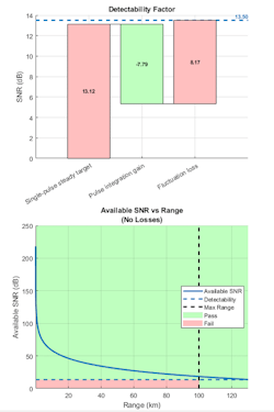
Figure 3 provides two types of plots for a visual framework to observe the results after each design tradeoff. The waterfall chart (top) illustrates the components of the detectability factor related to single-pulse operations, pulse integration gain, and target fluctuation loss. The stoplight chart (bottom) indicates we should be able to detect our target at 100 km.
The stoplight chart employs color-coded ranges and SNR levels according to the computed detectability. At the ranges where the available SNR curve passes through the green zone, the radar meets the detection requirement.
We know that for a fielded radar system, our design will have a shorter maximum range due to multiple factors including:
- Propagation effects caused by the earth’s surface and atmosphere, which reduce the amount of available signal energy at the receiver.
- Various losses experienced throughout the radar system.
Some of the most common losses are briefly described below.
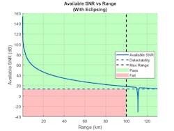
Pulse radar systems turn off their receivers during the pulse transmission. This means the target echoes arriving from the ranges within one pulse length from the radar or within one pulse length around the unambiguous range will be eclipsed by the transmitted pulse, resulting in only a fraction of the pulse being received and processed. This eclipsing effect results in the deep notch shown in Figure 4 at a range of ~110 km. Radar systems use pulse-repetition-frequency (PRF) diversity to prevent the eclipsing loss and extend the unambiguous range of the system.
A radar system can scan a search volume either by mechanically rotating the antenna or by using a phased-array antenna and performing electronic scanning. Imperfectly shaped antenna beams and the process of sweeping the beam across a search volume introduce additional losses to the system. Electronically steered phased arrays can impact the SNR due to beam broadening and a reduction in the effective aperture area of individual elements when steering off the radar boresight.
Prior to detection, the received radar echoes must pass through the radar signal-processing chain. The purpose of different components in the signal-processing chain is to guarantee the required probabilities of detection and false alarm, reject unwanted echoes from clutter, and account for non-Gaussian noise.
We need to consider several components of the signal-processing loss that must be accounted for in a surveillance radar system:
- Moving target indicator (MTI) is a process of rejecting fixed or slowly moving clutter while passing echoes from targets moving with significant velocities. Typical MTI uses a 2-, 3-, or 4-pulse canceller that implements a high-pass filter to reject echoes with low Doppler shifts. Passing the received signal through the MTI pulse canceller introduces correlation between the noise samples. This in turn reduces the total number of independent noise samples available for integration, resulting in MTI noise-correlation loss. In addition, the MTI canceller significantly suppresses targets with velocities close to the nulls of its frequency response, causing an additional MTI velocity-response loss.
- Binary integration is a suboptimal noncoherent integration technique also known as the M-of-N integration. If M out of N received pulses exceed a predetermined threshold, a target is declared to be present. The binary integrator, a relatively simple automatic detector, is less sensitive to the effects of a single large interference pulse that might exist along with the target echoes. Therefore, the binary integrator is more robust when the background noise or clutter is non-Gaussian. Since the binary integration is a suboptimal technique, it results in a binary integration loss compared with optimal noncoherent integration.
- Constant false alarm rate (CFAR) detection is used to maintain an approximately constant rate of false target detections when the noise or interference levels vary. Since CFAR averages a finite number of reference cells to estimate the noise level, the estimates are subject to an error, which leads to a CFAR loss. CFAR loss is an increase in the SNR required to achieve a desired detection performance using CFAR when the noise levels are unknown compared with a fixed threshold with a known noise level.
The scanning and the signal processing losses increase the detectability factor, which means that more energy is required to make a detection. The resulting detectability factor that includes the effects of all these losses is called the effective detectability factor. Figure 5 shows an updated waterfall chart and stoplight chart to reflect the types of losses described above.
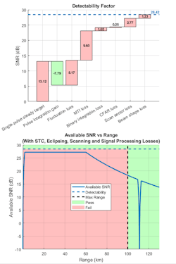
Note that in the stoplight chart, the SNR has now dropped into the red zone, which means when the losses are accounted for, the target will not be detectable.
What can we do to address this? We could boost transmit power or increase the antenna gains to bring up the available SNR. We could further increase the integration time to lower the required SNR. In some applications, some system parameters can be constrained by other requirements and thus are unable to be changed.
For example, if we’re considering changes to an existing system, increasing the available SNR might not be an option. Modifications to the signal-processing chain to lower the detectability factor may be the only acceptable solution.
To lower the required SNR, we could further increase the level of integration. Note that there’s a limit to increasing the number of integrated pulses. At some point, if the integration time is too long, the target will experience "range walk," where it will cross multiple range bins. Range walk can be an issue in imaging radars because it results in blurry returns.
We might also need to relax the requirements for the maximum range and the detection probabilities. For example, the Pd lower threshold value could be set to 0.8 (from 0.9). Similarly, the maximum-range requirement’s lower threshold value is set to 90 km (from 100 km). Figure 6 shows the updated SNR vs. range stoplight chart. Lowering the Pd from 0.9 to 0.8 will impact other requirement metrics, including probability of track, but this will be explored in a future blog.
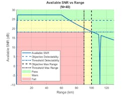
Now, the SNR vs. range plot has a yellow “Warn” zone indicating the SNR values and target ranges where system’s performance would be between our objective and the threshold requirements. We can see that up to approximately 70 km, the system meets the objective requirement for Pd. From 70 to 100 km, the objective requirement for Pd is violated while the threshold requirement is still satisfied.
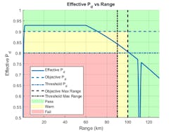
Figure 7 shows the plot of Pd as a function of range.
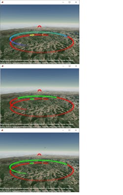
Now that we have the SNR and Pd detectability factor, let’s connect the analysis back to the terrain-based analysis we discussed in our earlier blog. To show this, let’s observe a small aircraft as it performs a corkscrew maneuver over mountainous terrain.
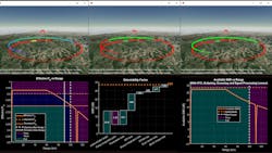
The radar location is shown on the maps in Figure 8 as a red semicircle. The left plot shows that the SNR of the received signals changes depending on where the aircraft is over the terrain. The red portion of the trajectory indicates that there’s no line-of-sight path between the aircraft and the radar, which means detection isn’t very likely.
We know that having line-of-sight doesn’t guarantee detectability. For our surveillance radar, we use pulse integration to reduce the required SNR similar to what we described earlier. In the center plot in Figure 8, the trajectory where the target is detectable is shown in green based on our minimum SNR requirement. Here, the red indicates no detectability.
In the right plot in Figure 8, we can see how increasing the transmitter power increases the region where the target is detectable. Notice that by increasing the peak power, the regions at the end of the trajectory that were previously undetected now satisfy the minimum SNR threshold.
To learn more about the topics covered in this blog and explore your own designs, see the examples below or email me at [email protected]:
- Radar Performance Analysis over Terrain (example): Learn how to analyze the performance of a ground-based, long-range terminal airport surveillance radar tasked with detecting an aircraft in the presence of heavy, mountainous clutter.
- Modeling Radar Detectability Factors (example): Learn how to model antenna, transmitter, and receiver gains and losses for a detailed radar range equation analysis.
- Radar Link Budget Analysis (example): Learn how to use the Radar Designer app to perform radar link budget analysis and design a radar system based on a set of performance requirements.
See additional 5G, radar, and EW resources, including those referenced in previous blog posts.
Rick Gentile is Product Manager, Sara James is Senior Software Developer, Peter Khomchuk is Senior Software Engineer, and Honglei Chen is Principal Engineer at MathWorks.
About the Author
Rick Gentile
Product Manager, Phased Array System Toolbox and Signal Processing Toolbox
Rick Gentile is the product manager for Phased Array System Toolbox and Signal Processing Toolbox at MathWorks. Prior to joining MathWorks, Rick was a radar systems engineer at MITRE and MIT Lincoln Laboratory, where he worked on the development of several large radar systems. Rick also was a DSP applications engineer at Analog Devices, where he led embedded processor and system level architecture definitions for high performance signal processing systems used in a wide range of applications.
He received a BS in electrical and computer engineering from the University of Massachusetts, Amherst, and an MS in electrical and computer engineering from Northeastern University, where his focus areas of study included microwave engineering, communications, and signal processing.
