Algorithms to Antenna: Where Should I Locate My Radar?

In a previous blog, we wrote about ways to visualize antenna patterns on a map. We want to revisit this topic by sharing another example related to planning a small network of radar systems. First, a bit of background.
The Engineering Research Center for Collaborative Adaptive Sensing of the Atmosphere (CASA) at the University of Massachusetts Amherst has described a concept in which new gap-filling radars could be used to augment existing radar networks. The types of radars they envision are low-power, phased-array systems that can be used to detect aircraft as well as make weather observations. The impetus behind this work is the advent of smaller aircraft and drones that may be too small to be reliably detected with existing radar systems.
When we think of small air vehicles that could fly through an air space, a radar cross-section (RCS) of 0.1 square meters is realistic. These types of platforms can fly much closer to the ground, which also makes detection more challenging.
When modeling this type of system, we want to increase the probability of detecting small aircraft at long distances from the radar (up to 35,000 meters in this example). This should be accomplished by installing additional radars to augment an existing network.
Each of these radars has highly directional phased-array antennas. If we assume some amount of pulse integration at the radar receiver, the required signal-to-noise ratio (SNR) level to achieve detections is lowered, which can help keep the transmitter power at a reasonable level. For example, integrating 10 pulses noncoherently results in an SNR level of about 5 dB to detect a small target (Fig. 1). This results in transmit power levels that are measured in tens of watts.
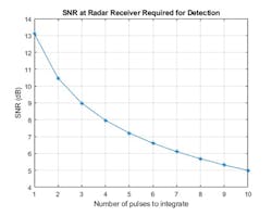
1. The SNR at the radar receiver required for detection of a small object is plotted.
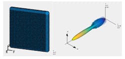
Figure 2 shows an antenna array of an X-band radar that’s small enough to be easily mounted on a variety of support structures. The smaller form factor makes deploying this type of system much easier. The antenna-array pattern from this design can be directly used in a radar planning workflow.
For our hypothetical radar network, we have five candidate locations to place our low-power radars. Our goal is to select the three best locations for installation.
We first define a scene that includes DTED level-1 terrain data. We start with the radar equation and calculate additional path losses due to terrain obstruction and diffraction. For this, we can use either the Longley-Rice propagation model or the Terrain Integrated Rough Earth Model (TIREM).
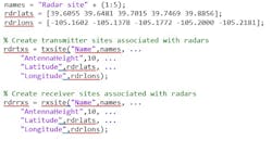
Our network is based on a region around Boulder, Colorado. The terrain file was downloaded from the "SRTM Void Filled" data set available from the United States Geological Survey (USGS). The file—DTED level-1 format—has a sampling resolution of about 90 meters. Note that a single DTED file defines a region that spans one degree in both latitude and longitude. The code to bring the data into MATLAB is as follows:

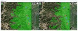
In Figure 3, one can see that the region contains mountains to the west and flatter areas to the east. Our radars will be placed in the flat terrain to detect targets over the mountainous region. The candidate locations are chosen to correspond to local high-elevation points on the map outside of residential areas. Each radar is assumed to be 10 meters above ground level.
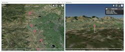
3. Five candidate radar locations are revealed on the left, while a view of terrain from one of the radar locations is shown on the right.
The MATLAB code used to set up the radar transmitter and receiver is as follows:
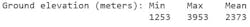
Our region of interest, which spans 0.5 degrees in both latitude and longitude, includes mountains to the west as well as some of the area around the radar sites. The goal is to detect targets that are in the mountainous region to the west. For this region of interest, the summary elevation is:
The altitude of aircraft in the radar coverage can be defined with respect to either mean sea level or ground level. For the purposes of this example, a target is detected if the radar receiver SNR exceeds the SNR threshold required for a detection, which we have calculated to be 5 dB. Using a simple form of optimization, all combinations of radar sites are considered. We can then select the three sites that produce the highest number of detections from the coverage. Figure 4 shows the results for the cases in which the aircraft are 500 m and 250 m above the ground.
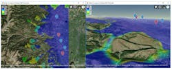
4. The blue markers indicate the three best locations for radar installation for targets at 500 m above ground (left) and 250 m above ground (right).
The three radar sites selected for best coverage are indicated with blue markers. The coverage map shows straight edges on the north, east, and south sides corresponding to the limits of the region of interest. We assume the radars can rotate (or be electronically steered) to produce the same antenna gain in all directions, and they can transmit and receive simultaneously so that there’s no minimum coverage range.
The coverage map has jagged portions on the western edge where the coverage areas are limited by terrain effects. A smooth portion of the western edge appears where the coverage is limited by the design range of the radar system, which is 35,000 meters. It’s also interesting to consider the case when the target position is 250 meters above ground level (versus 500 meters above ground level in the previous view). As expected, the coverage map in Figure 4 shows that reducing the visibility of the targets also decreases the coverage area.
Figure 5 illustrates how this same type of scenario can also be visualized with different SNR thresholds to gain better insights into the network’s performance.
5. This coverage map presents different SNR levels from a bird’s-eye view and from a target perspective.
Integrating terrain into a radar coverage map can help with analysis and planning activities. This type of workflow also can save field work. Moreover, it may help in the iterative radar design in terms of power, array size, and signal processing.
To learn more about the topics covered in this blog, see the links below or email [email protected].
- Planning Radar Network Coverage over Terrain (example): Learn how to plan a radar network using propagation modeling over terrain.
- Simulating a Polarimetric Radar Return for Weather Observation (example): Learn how to simulate a polarimetric Doppler radar return that meets the requirements of weather observations.
- Designing a Basic Monostatic Pulse Radar (example): This example shows how to design a monostatic pulse radar to estimate the target range.
See additional 5G, radar, and EW resources, including those referenced in previous blog posts.

About the Author
Rick Gentile
Product Manager, Phased Array System Toolbox and Signal Processing Toolbox
Rick Gentile is the product manager for Phased Array System Toolbox and Signal Processing Toolbox at MathWorks. Prior to joining MathWorks, Rick was a radar systems engineer at MITRE and MIT Lincoln Laboratory, where he worked on the development of several large radar systems. Rick also was a DSP applications engineer at Analog Devices, where he led embedded processor and system level architecture definitions for high performance signal processing systems used in a wide range of applications.
He received a BS in electrical and computer engineering from the University of Massachusetts, Amherst, and an MS in electrical and computer engineering from Northeastern University, where his focus areas of study included microwave engineering, communications, and signal processing.
Jacob Halbrooks
Senior Software Engineer
Honglei Chen
Principal Engineer
Honglei Chen is a principal engineer at MathWorks where he leads the development of phased-array system simulation. He received his Bachelor of Science from Beijing Institute of Technology and his MS and PhD, both in electrical engineering, from the University of Massachusetts Dartmouth.
