Accurate Models and Discrete Part-Value Optimization Combine to Improve Workflows

Download this article in PDF format.

Designing RF filters and other high-frequency circuits with today’s simulation software tools often involves performing some form of optimization to achieve the desired performance. For example, take the case of a lumped-element filter. Optimizing such a filter involves adjusting the values of its lumped components until the filter achieves an optimal frequency response.

However, once the component values have been determined via optimization, they may still need to be adjusted to the closest discrete, or “real-life,” manufacturer part values. Depending on the design’s complexity, this extra step can create a bit of extra legwork for the designer.

Of course, additional simulations must be performed after changing the optimized part values to the nearest available manufacturer part values. And if an optimized value falls roughly halfway between the two closest available manufacturer part values, one may need to experiment to determine which of the two values allows for better performance. In such cases, designers may need to carry out further refinements by adjusting interconnect dimensions to fine-tune the filter performance after setting the component values to the closest available manufacturer part values.

Fortunately, with the proper tools, it’s possible to perform discrete part-value optimizations in which component values are directly adjusted to optimal manufacturer part values. This optimization method eliminates the need for designers to manually adjust optimized component values to the closest available real-life part values, thereby cutting one step from the overall design process.

This article explains how a discrete part-value optimization method can be leveraged to develop a lumped-element bandpass filter designed using the Cadence AWR Design Environment (AWRDE). The design includes Modelithics measurement-based passive-component models, which enable simulations to accurately predict the filter’s real performance. After completing an initial filter design, a discrete part-value optimization achieves the desired frequency response. The article wraps up by comparing measured data to the simulated results.

Beginning with the iFilter Synthesis Module

The AWRDE consists of several software tools used for developing RF/microwave products. Among them are Microwave Office for RF/microwave circuit design and the AXIEM 3D planar electromagnetic (EM) simulator. For this design example, we used both of these tools.

Various add-on modules can also be utilized within the AWRDE platform. One of them is iFilter, an integrated synthesis wizard used to develop RF/microwave filters. With iFilter, designers can synthesize lumped-element and distributed filters and then directly export them to Microwave Office for further analysis.

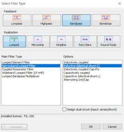
For this example, we used iFilter to start the design process. Users open the iFilter module within AWRDE by double-clicking iFilter Filter Synthesis, which is located under Wizards in the Project browser. Starting a new filter design with iFilter prompts users to specify the type of filter desired by selecting a Passband, Realization, Main Filter Type, and Options (Fig. 1). For this example, we specified the Passband as Bandpass and the Realization as Lumped. Following these selections, we chose Narrowband Lumped Filter as the Main Filter Type. Subsequently, we selected Inductive (identical shunt C) from the list of options.

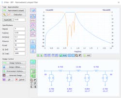
1. This is the user interface when starting a design with iFilter.

Specifying the type of filter leads to the next user interface, which contains the filter schematic, frequency response, and several user-defined parameters (Fig. 2). For this design example, we specified a Chebyshev filter with a center frequency of 950 MHz and bandwidth of 300 MHz.

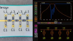
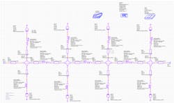
2. Users can specify the filter parameters via this interface, which also illustrates the frequency response and filter schematic.

Clicking Generate Design automatically creates a new schematic of the filter in Microwave Office (Fig. 3). Note that the tool automatically set several variables.

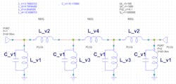
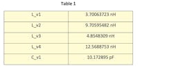
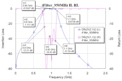
3. Using iFilter to generate the filter design results in this Microwave Office schematic. The bold reference designations that correspond to the variables were added for illustration purposes.

The bold reference designations that correspond to the variables were added to the schematic for illustration. In this case, the variable C_v1 was created for all capacitor values, while variables L_v1, L_v2, L_v3, and L_v4 were created for all inductor values. Table 1 lists these variables and their corresponding values; Figure 4 shows the filter’s simulated frequency response.

These variables generated by iFilter represent the part values of the inductors and capacitors.

4. The simulated frequency response reveals a center frequency of 950 MHz.

Incorporating Microstrip Transmission Lines and Modelithics Models

While the schematic shown in Figure 3 represents a good starting point for the design, the overall design process is far from complete. For one, to properly model a real filter, one must add microstrip interconnects to the schematic. Adding the microstrip interconnects makes it possible to generate a layout that can later be sent to a printed-circuit-board (PCB) manufacturer for fabrication.

We must also consider component modeling. In the schematic shown in Figure 3, the inductor and capacitor models are ideal closed-form elements with user-defined quality-factor (Q) parameters.

Alternatively, utilizing Modelithics measurement-based inductor and capacitor models makes it possible to predict the filter’s performance more accurately. The company’s models offer the benefit of both part-value and substrate scalability. These models accurately capture substrate-dependent parasitic behavior and offer advanced pad features for accurate EM/circuit co-simulations. Hence, we used Modelithics inductor and capacitor models in place of the ideal elements seen in Figure 3.

Of course, one could simply modify the original schematic by adding the microstrip transmission lines and the Modelithics models. Another approach—and the one used in this case—is to duplicate the original schematic, leaving it extant as a reference if needed. Figure 5 shows a new filter schematic created by duplicating the original one. This new schematic contains all the necessary microstrip interconnects and vias. In addition, the ideal inductor and capacitor models are replaced with the company’s models.

5. The new filter schematic incorporates microstrip interconnects and vias along with Modelithics passive-component models.

For this example, the Würth Elektronik WE-KI 0402-size inductors are chosen for all the inductors. For the capacitors, Kemet’s CBR04C 0402-size capacitors are used. Furthermore, the substrate used for this filter is 10-mil-thick Rogers RO4350B, which was implemented by placing the corresponding Modelithics substrate definition on the schematic.

The schematic shown in Figure 5 also includes an EXTRACT block and a STACKUP multi-layer substrate definition. We added these elements to the schematic via the Create_Stackup script, which can be accessed by selecting Scripts from the toolbar followed by EM>Create_Stackup. These two elements together facilitate EM/circuit co-simulation by creating and configuring a metal geometry from the PCB layout of selected schematic elements.

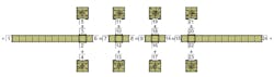
In this case, we selected all of the microstrip interconnects and vias for extraction. Therefore, these elements will be analyzed with the AXIEM EM simulator. The inductors and capacitors are the only elements from the schematic that aren’t extracted for EM analysis, because they will be analyzed within the Microwave Office circuit simulator. Figure 6 shows the extracted EM structure comprising all the interconnects and vias.

6. We extracted this EM structure with the help of the Create_Stackup script.

Now that the EM extraction is properly configured, we can perform an EM/circuit co-simulation by simulating the schematic shown in Figure 5. As explained above, the microstrip interconnects and vias will be analyzed with the AXIEM EM simulator, while the components will be analyzed within the Microwave Office circuit simulator. Also, this schematic includes the same variables found in the original schematic (Table 1, again). The inductor and capacitor values of the Modelithics component models are set to the same variables as the corresponding components in the original schematic, meaning the component values are unchanged.

Some designers may want to see how the microstrip interconnects alone affect the filter’s performance. To do so, set the Sim_mode parameter of all Modelithics models to 1. Setting a model’s Sim_mode parameter to 1 enables it to simply behave as an ideal element, meaning that real-world parasitic, pad, and substrate effects are not considered. Thus, utilizing this setting for all models makes it possible to determine how the microstrip transmission lines alone affect performance, because the design is still employing ideal component models like the original schematic.

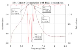
Figure 7 shows the simulated performance of the filter with the Sim_mode parameter set to 1 for all models. Notice how the response is shifted downward in frequency in comparison to the original frequency response (Fig. 4, again).

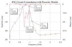
7. Shown is the simulated S21 and S11 with the Sim_mode parameter of all the Modelithics models set to 1. The results show that adding the microstrip elements resulted in a downward shift in frequency in comparison to the original frequency response.

We can now set the Sim_mode parameter of all models to 0. This setting enables a model to behave as a full parasitic model, thus accounting for all real-world parasitic, pad, and substrate effects. Figure 8 shows the frequency response after simulating the filter with Sim_mode set to 0 for all models. It’s evident that the response shifted further downward in frequency and is more lossy compared to the results shown in Figure 7. Specifically, the center frequency of the passband is approximately 800 MHz, a 150-MHz shift from the desired center frequency of 950 MHz. The filter also falls short of achieving the desired 300-MHz bandwidth.

8. After setting Sim_mode to 0 for all Modelithics models, the filter shifts further downward in frequency and exhibits greater passband insertion loss.

Discrete Part-Value Optimization to the Rescue

Because the filter doesn’t currently meet the design goals, the next step is to perform a discrete part-value optimization. This optimization technique will directly adjust the inductor and capacitor values to the optimal part values in the Würth Elektronik WE-KI and Kemet CBR04C part families, respectively.

To facilitate performance of discrete part-value optimizations in the AWRDE, Modelithics offers .txt files for all passive-component models. Each file contains a list of all manufacturer part values in the part family represented by the model. These files are located in the <installDir>\Modelithics\Data folder, where <installDir> is the installation folder (C:\Program Files (x86)\AWR\Foundry by default). The IND_WTH_0402_002.txt file contains all part values in the Würth Elektronik WE-KI family of inductors, while the CAP_KMT_0402_004.txt file contains the same information for the Kemet CBR04C capacitor family.

Figure 9 displays the equations that must be added to the Microwave Office schematic (Figure 5, again) to utilize these files for a discrete part-value optimization. The equations shown are based on the default file locations. Note that the IND_WTH_0402_002.txt and CAP_KMT_0402_004 .txt files generate two vectors, L_vector and C_vector, respectively. As a result, the L_vector element contains each of the part values in the Würth Elektronik WE-KI part family, while the C_vector element contains each of the part values in the Kemet CBR04C part family.

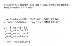
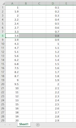
9. Adding these equations to the Microwave Office schematic enables the appropriate .txt files to be the basis for a discrete part-value optimization.

From the values shown in the bottom portion of Figure 9, we can see that the variables are no longer equal to the initial values of Table 1. Rather, they’re now set to the vector indices that correspond to the manufacturer part values closest to the initial values. Users may easily determine these indices by copying the part values from the .txt files and pasting them into a spreadsheet (Fig. 10).

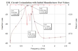
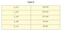
10. We can copy the part values from the .txt files and paste them into a spreadsheet (columns A and D) to determine the vector indices.

Simulating the filter produces the frequency response shown in Figure 11. The results are similar—but not quite identical—to the simulated results of the filter with the initial part values (Fig. 8, again). Table 2 lists the manufacturer part values used for this initial simulation.

11. Changing the filter’s initial part values to the closest manufacturer part values results in the frequency response shown.

Shown are the manufacturer part values that are closest to the initial values.

It’s now time to perform a discrete part-value optimization. To do so, we specify the variables L_v1, L_v2, L_v3, L_v4, and C_v1 for optimization in the Variable Browser (Fig. 12). Next, we set the optimization goals. Over the passband of 800 to 1100 MHz, we’re shooting for an S₂₁ value greater than −2 dB and an S₁₁ value less than −12 dB. For the lower and upper rejection bands, the goal is an S₂₁ value of less than −20 dB. Finally, upon opening the optimization user interface, the user must select Discrete Local Search from the list of optimization methods.

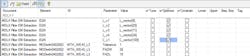
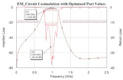
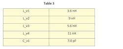
12. To execute a discrete part-value optimization, the variables that represent the part values of the inductors and capacitors must be specified for optimization in the Variable Browser.

Figure 13 shows the filter’s simulated frequency response after performing the discrete part-value optimization, while Table 3 lists the optimized manufacturer part values. Now that the filter performs well, the design process is complete. Keep in mind that one may fine-tune interconnect dimensions to tweak a design so as to achieve the desired performance. In this case, that step wasn’t necessary.

13. Shown is the filter’s post-optimization frequency response. The response reveals a center frequency of 950 MHz along with the desired bandwidth.

These are the final optimized manufacturer part values.

Measured Data Versus Simulated Results and Closing

The final step is to validate the design by building and measuring the filter. We assembled two filters using the same Würth Elektronik WE-KI inductors and Kemet CBR04C capacitors from the final simulation (Fig. 14).

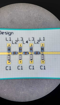
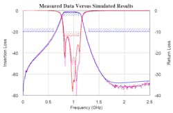
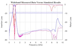
14. Shown is one of two filters built with the same Würth Elektronik inductors and Kemet capacitors from the simulation.

Figure 15 shows the measured data of both filters along with the final simulated results. The measured data agrees with the simulated results, thereby validating the design process. Figure 16 reveals the simulated results and measured data over a wider frequency range.

15. The measured data for S21 and S11 (dashed traces) largely agreed with the corresponding final simulated results (solid traces).

16. Shown are the measured data (dashed traces) and simulation results (solid lines) over a wide frequency range.

In closing, utilizing Modelithics measurement-based models combined with a discrete part-value optimization method within the Cadence AWR Design Environment can be an effective way to design RF/microwave circuits. The approach pinpoints exactly which manufacturer part values are best suited for a design.

Chris DeMartino is a Sales and Applications Engineer at Modelithics Inc.