EM Co-Simulation with Measurement-Based Models Leads to First-Pass Design Success
Download this article in PDF format.
When simulating high-frequency filters with discrete passive components, it’s important to consider several factors to achieve simulation results that correspond to actual measured performance. One such aspect is the metallization that connects components together, as these metal interconnects impact the overall filter performance. In addition, component parasitics should be incorporated into a simulation to ensure that the simulated results accurately predict the filter’s response.
Fortunately, electromagnetic (EM) simulation software, such as Sonnet Suites from Sonnet Software, makes it possible to incorporate metal interconnects into a simulation. However, EM simulations that include ideal passive-component models often expose a discrepancy between simulated and measured performance, because ideal component models don’t account for the parasitics that are present in real-world parts.
To help overcome these challenges, Modelithics offers measurement-based passive-component models that aid filter designers who use discrete passive components. These part-value, scalable models accurately capture substrate-dependent parasitic behavior so that they serve as true representations of real-world components in the context of their physical environment. Thus, incorporating Modelithics passive-component models into a filter simulation helps to accurately predict real-world performance and achieve first-pass design success.
Modelithics Microwave Global Models are available for use with various simulation software tools, including Sonnet Suites. In addition to part-value and substrate scalability, these models offer advanced pad features that facilitate accurate EM co-simulations.1 Designers can therefore utilize the combination of Modelithics models and Sonnet’s EM solver to account for real-world component parasitics and metal interconnects in a simulation.
To demonstrate this combination, this article presents a workflow for a fifth-order Butterworth bandpass filter that features Modelithics passive-component models and Sonnet’s EM software. Measured data is presented at the conclusion to compare simulation versus measurement results.
Starting with a Lowpass Prototype
As stated, the filter that will be designed here is a fifth-order Butterworth bandpass implementation. Intended for GPS applications, the filter provides lower and upper cutoff frequencies of 1,050 and 1,700 MHz, respectively, thereby allowing it to pass the L1, L2, L3, and L5 GPS bands.
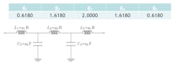
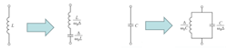
The design process begins by determining the coefficients for a maximally flat, five-element lowpass filter with ωc = 1 rad/s and RS = RL = 1 Ω.2 This lowpass prototype will later be transformed to a bandpass network. Figure 1 displays the coefficient values for the maximally flat, five-element lowpass prototype filter along with the corresponding schematic. Note the symmetry in the g values, which results in fewer unique component values in the filter design.
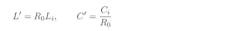
Because the filter is being designed for a 50-Ω reference environment, the coefficients must be scaled in impedance based on the following equations:
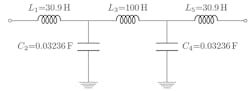
Applying these equations to the filter shown in Figure 1 results in a new 50-Ω-referenced filter with updated component values (Fig. 2).
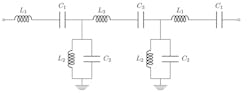
The lowpass filter prototype must now be converted to a bandpass implementation via frequency mapping. This conversion involves transforming the series inductors to series-LC circuits, while the shunt capacitors are transformed to parallel-LC circuits. Figure 3 illustrates the element transformations.
In Figure 3, note that:

and:

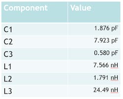
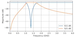
Figure 4 depicts the schematic of the bandpass filter that’s produced after transforming the lowpass prototype; its derived component values appear in Table 1. Furthermore, Figure 5 below plots the filter’s calculated frequency response.
Creating the Design in Sonnet Suites
After determining the ideal component values of the bandpass filter, the next step is to create the design using the Sonnet Project Editor. Be aware that the calculated frequency response shown in Figure 5 didn’t account for the metal interconnects that will be present in the real-world filter. In contrast, creating the design in Sonnet Suites makes it possible to include these interconnects in the simulation.
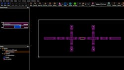
For this design, we chose 10-mil-thick Rogers RO4350B laminate as the substrate. Figure 6 shows the filter layout in the form of a CAD (DXF) file, which was ultimately sent to a printed-circuit-board (PCB) manufacturer for fabrication. In this case, the line widths are set to 21.7 mils. One can clearly see the various gaps between traces that indicate component locations on the PCB.
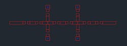
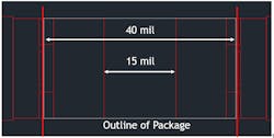
It’s important to point out that what’s simulated must replicate what will eventually be built. Therefore, when simulating the filter in Sonnet, one should ensure that the component models are attached to the correct reference planes in the filter geometry. A gap of 15 mils between pads is included in the default pad arrangement for the filter’s 0402-size components.
Because the 40-mil-long parts will be centrally placed on the pads, the ports must be broken out 12.5 mil into each pad to coincide with the edge of the part (12.5 + 15 + 12.5 = 40). Figure 7 presents a depiction of this arrangement. This example illustrates the advanced pad features of the Microwave Global Models, which provide the needed flexibility for placement of the reference planes.
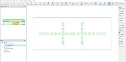
Now, we can use Sonnet Suites to import the DXF file of the filter layout. During the importation process, users can specify the layer mapping followed by the box size and cell size. Sonnet also provides users with options for importing vias.
Figure 8 shows the Sonnet project after successfully importing the layout. The left-hand side of the Sonnet interface contains the Stackup Manager, which is where one may specify vias and top-layer metal (FRONTMETAL). We specified the top dielectric, which is set to air by default, for a thickness of 100 mils to minimize the shielding effect of the lossless metal top cover. Lastly, we added ports to the conductor edges where the filter’s input and output are located. In this case, we used the default port settings.
Simulating with Ideal Component Models
Next, the component models are added to the Sonnet project. Before adding the models, we created variables for each of the component values derived earlier (Table 1, again). In this case, we added variables for C1, C2, C3, L1, L2, and L3, with each one assigned its corresponding part value. In addition, each variable must be specified as optimizable, with the optimization range set to the range of part values for the corresponding part family (the part families will be revealed later). We set these variables to be optimizable because the filter will eventually require tweaking to achieve the desired performance.
Now we add the Modelithics component models to the design. Users can choose from a wide range of models that can be sorted either by type or by vendor. For this design, we chose the TDK MHQ1005P inductor part family for all inductors and the Kemet CBR04C part family for all capacitors.
An important parameter to note for a Modelithics component model is Sim_mode. For this initial simulation, Sim_mode is set to 1 for all component models. This setting allows a component model to simply behave as an ideal element, meaning that real-world factors like parasitic, pad, and substrate effects aren’t considered. Furthermore, each model’s value is set to the corresponding variable created earlier.
By executing a simulation with the Sim_mode parameter of all component models set to 1 for ideal mode, one may determine the performance impact of the metal interconnects (microstrip lines) themselves. In other words, the metallization incorporated into the Sonnet project represents the only real difference between this filter design with ideal models and the initial filter schematic shown earlier (Fig. 4, again). To determine the impact of metallization on performance, it’s a simple matter of comparing the simulation results to the initial calculated frequency response (Fig. 5, again).
Before simulating, we specified a linear frequency sweep from 0.05 to 10 GHz with 401 measurement points. In addition, we selected the Adaptive option to improve the simulation time by interpolating solutions when appropriate.
Figure 9 shows the results of the Sonnet simulation with ideal component models (blue and red traces). For comparison purposes, Figure 9 also displays the calculated frequency response of the initial filter schematic shown in Figure 5, which didn’t account for the physical effects of metal traces (dashed black traces). The Sonnet simulation predicts a response that’s shifted downward in frequency compared to the response of the initial filter. In addition, the passband response is obviously not flat. Thus, we must optimize the filter to obtain the ideal component values that result in the filter’s optimal performance.
Performing an optimization requires defining one or more sets of optimization goals. In this case, we defined three sets of goals. For the passband, the optimization goals are an S21 value greater than −1 dB and an S11 value less than −10 dB. For the lower and upper rejection bands, we’re shooting for an S21 value of less than −20 dB.
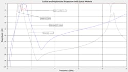
Figure 10 shows the simulated results of the optimized filter along with the results of the previous Sonnet simulation with the initial component values. The filter’s response is now shifted upward in frequency to correspond with the design goals. In addition, we’ve achieved the desired flat passband. Table 2 shows the values of the optimized filter’s ideal components. (It should be noted that this step of performing an optimization with ideal models isn’t necessary, but it’s included here to illustrate the progression of part-value changes as more and more real-world effects are included).
Moving from Ideal to Real-World Component Models
Optimizing the filter using ideal component models is a good starting point for determining the final component values. However, there’s room for improvement, because the ideal component models didn’t account for real-world parasitic and substrate effects. Therefore, the next step is to update the component models to include these effects, providing an even more accurate prediction of the manufactured circuit’s behavior.
Incorporating parasitic and substrate effects into a Modelithics model requires setting its Sim_mode parameter to the proper value. To include these effects, the Sim_mode parameter can now be set to 2 for all models. Note that with this setting, pad effects are removed (i.e., de-embedded) from a Global model. In this case, it’s correct to employ this setting because the pads are already accounted for in the EM simulation. However, we can enable pad effects by setting a model’s Sim_mode parameter to 0.
Because the component models now account for parasitic and substrate effects, they essentially represent real-world components rather than ideal ones. The next step is to perform a simulation with these models while leaving their inductance and capacitance values unchanged from the optimized filter with ideal component models. Figure 11 shows the results of this simulation (blue and red traces). For comparison, we again show the response of the optimized filter that contains ideal component models with identical values (dashed black traces).
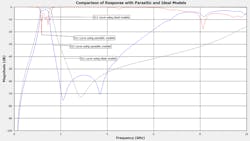
Neglecting to account for parasitic effects in a simulation can lead to simulated results that deviate significantly from real-world performance (Fig. 11, again). It’s clear that simulating the filter with the real-world models resulted in a passband response that’s both narrower and more lossy than the passband response of the filter with ideal component models having equivalent inductance and capacitance values. Thus, a filter manufactured using components with the same values as the ideal component models would not achieve the design goals.
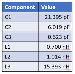
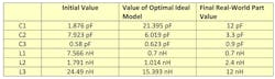
To meet the design goals, we must perform a final step of optimizing the filter with the parasitic effects included. For this optimization, we use the same optimization goals specified earlier. Note that once the optimization is complete, the component values must be changed to the closest available discrete, or “real-life,” part values available in the given component family. These real-life values correspond to the values of the real inductors and capacitors that will be used when building the filter.
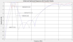
Figure 12 shows the final simulated results of the optimized filter using parasitic models with real-life values. These values, listed in Table 3, resulted from adjusting the optimized component values to the closest available manufacturer part values.
For comparison, Table 3 also shows the component values of the optimized filter with ideal models along with the initial component values.
As Figure 12 demonstrates, the filter now achieves the desired performance. Further refinements could be made by adjusting lengths and widths of the interconnects to fine-tune the filter performance after the component values are set to the closest available manufacturer part values.
Measured Data and Closing
To validate the simulated results, we built and measured three filters (Fig. 13). We populated the filter PCBs with the same TDK inductors and Kemet capacitors from the final simulation and probed all measurements. Through a thru-reflect-line (TRL) calibration, we moved the reference planes to match those used in the simulation.
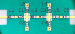
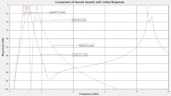
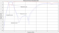
Figure 14 shows the measured data from one of the filters we built (dashed traces) along with the results of the final simulation (solid traces). It’s clear that the measured 3-dB frequencies, as well as the S21 and S11 values within the passband, are almost identical to the simulated results, thus validating the workflow presented.
In closing, the combination of Modelithics measurement-based models and Sonnet’s EM simulator represents an effective way to design high-frequency filters with discrete passive components. The example highlighted in this article demonstrates that incorporating Modelithics models into a Sonnet project can help achieve first-pass design success. In contrast, simulating high-frequency filters with ideal passive-component models can create headaches for designers, because the simulated results may not be a true indication of the filter’s performance.
Acknowledgement
The authors would like to thank Greg Kinnetz of Sonnet Software for his support.
Eric Valentino is an RF Engineer, and Chris DeMartino is Sales and Application Engineer at Modelithics.
References
1. See related Modelithics application notes at https://www.modelithics.com/Literature/AppNote, especially 37, 39, 48, 51, 57, 60, and 61 .
2. Matthaei, Young, and Jones, Microwave Filters, Impedance-Matching Networks, and Coupling Structures, 1980.
3. DeMartino C., “Take the Guesswork Out of Discrete Circuit Design,” Microwaves & RF, December 2018.
About the Author
Eric Valentino
RF Engineer, Modelithics
Eric Valentino graduated with a Master’s in Electrical Engineering in August of 2019, while working as an Engineering Intern with Modelithics. Upon graduation, he was brought on full-time as an RF Engineer/EM Specialist with Modelithics, utilizing his experience with multiple full-wave electromagnetic analysis tools involving both finite element method (FEM) and Method of Moments (MoM) solutions. He also has experience with planar circuit simulators and complex scalable models and model libraries for both circuit and EM simulators. Eric is currently focusing on expanding Modelithics’ library of 3D component models as well as contributing to a team responsible for automation of various processes at Modelithics.
