Algorithms to Antennas: Simulate and Track Targets in Terrain-Based Scenarios
This blog is part of the Algorithms to Antennas Series
What you'll learn:
- Modeling surveillance radar with two targets.
- What happens when the targets are occluded by terrain?
- Results obtained when executing a full simulation.
In our recent blog, we focused on improving the fidelity of radar simulations by increasing the fidelity of how land and sea surfaces are modeled.
This article leverages one of the techniques described in the blog referenced above. For our example, we model a surveillance radar set in a mountainous region where the terrain can occlude both ground vehicles and low-altitude aerial vehicles.
Using this type of model can help with evaluating new system designs in addition to upgrades in existing systems. It also can help you understand performance-related parameters for your radar system, as well as where to locate the radar system to maximize detectability.
Surveillance Model Example with Two Targets
We start with a geo-referenced location using terrain data from a Digital Terrain Elevation Data (DTED) file. For the example that follows, the DTED spans latitude between 39 and 40 degrees North and longitude between 105 and 106 degrees West, which corresponds to a mountainous region in Colorado, USA.
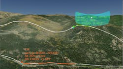
Our scenario (Fig.1, left) includes a surveillance radar and two targets. In the model, we mount the surveillance radar on a tower. The tower, located on top of a mountain, searches the area where the two targets traverse. The first target is a drone flying at an altitude 20 meters above the terrain height. The second target is a ground vehicle that follows a road through a mountain pass.
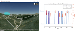
We know that the radar will have a difficult time seeing the targets when they’re occluded by terrain. In the right side of Figure 1, the left axis of the plot shows the occlusion status of each target over time. With this information, you can see when radar detections aren’t available. The radar tracker uses detections to form tracks and we apply a tracking metric to measure the effectiveness of the radar system for this scenario.
The optimal subpattern assignment (OSPA) metric is computed for our set of tracks and the known truths. On the right axis of the plot, you can see the quantitative assessment of the tracker performance. The tracking performance correlates directly with the occlusion status. Note that for the OSPA score, lower is better. As expected, the radar isn’t able to track targets when they’re occluded.
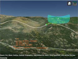
Figure 2 shows a segment of the simulation after ~100 seconds. This corresponds to the time that the drone enters the occluded area at the foot of the mountain. Notice that the track is coasted, and its associated uncertainty grows due to the lack of observations until it’s eventually deleted. The previous OSPA plot slowly increases during coasting before jumping to the threshold value upon track deletion. In the meantime, the ground vehicle, traveling on the road, is occluded and therefore undetected.
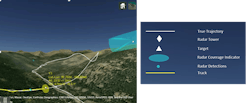
Figure 3 shows the same simulation after 155 seconds. The drone and ground vehicle are no longer occluded, as shown in the occlusion state plot, except for a moment when the drone passes by the saddle point in between mountains. The track is briefly coasted and recovered with the next available radar detections.
This period of the simulation also is noticeable on the occlusion and OSPA plot. The performance starts to degrade (OSPA value increases) after the occlusion status switches, but it recovers immediately when the status switches again.
Full Simulation Results
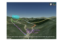
Figure 4 shows the results over the full simulation. The tracks exist for each target when the terrain doesn’t occlude the line of sight. The true trajectories of the ground target and the drone are displayed in white. The generated tracks are represented by colored lines. The three segments of the drone track are shown in yellow, green, and purple. The ground vehicle tracks are shown in blue and orange.
In this particular scenario, the long occlusion time makes it difficult for the tracker to maintain a unique track ID for each target. It might require either more radar systems that can provide better coverage overall, or a different location for the existing radar to improve detectability for this region. Alternatively, a map-aware tracker or a tracker that uses target features like the drone’s micro-Doppler signature could be used to improve tracker ability to coast and reacquire the target.
This workflow can be applied using terrain data from other DTED files. You can change the radar design or change the targets and target trajectories to match your own system.
One more note. This will be the final blog that our colleague Rick Gentile will be authoring. It has been a pleasure working with Rick on this series. We will carry the series forward with similar topics we think you will find helpful and interesting. To learn more about the topics covered in this blog and explore your own designs, see the examples below or email me at [email protected].
Rick Gentile is Product Manager, Gael Goron is Senior Software Developer, Elad Kivelevitch is Senior Team Lead, Vincent Pellissier is Engineering Manager, and Honglei Chen is Principal Engineer at MathWorks.
- Simulate and Track Targets with Terrain Occlusions (Example code): Learn how to model a surveillance scenario in a mountainous region where terrain can occlude both ground and aerial vehicles from the surveillance radar.
- Introduction to Radar Scenario Clutter Simulation (Example code): Learn how to generate monostatic surface clutter signals and detections in a radar scenario.
- Simulate and Track En-Route Aircraft in Earth-Centered Scenarios (Example code): Learn how to model a system that uses a monostatic radar detections and ADS-B reports to track aircraft.
See additional 5G, radar, and EW resources, including those referenced in previous blog posts.
Read more blogs in the Algorithms to Antennas Series
About the Author
Rick Gentile
Product Manager, Phased Array System Toolbox and Signal Processing Toolbox
Rick Gentile is the product manager for Phased Array System Toolbox and Signal Processing Toolbox at MathWorks. Prior to joining MathWorks, Rick was a radar systems engineer at MITRE and MIT Lincoln Laboratory, where he worked on the development of several large radar systems. Rick also was a DSP applications engineer at Analog Devices, where he led embedded processor and system level architecture definitions for high performance signal processing systems used in a wide range of applications.
He received a BS in electrical and computer engineering from the University of Massachusetts, Amherst, and an MS in electrical and computer engineering from Northeastern University, where his focus areas of study included microwave engineering, communications, and signal processing.
