All About Circular Polarization and the Axial Ratio

What you’ll learn:

• The nature of different antenna polarizations.
• Circular polarization and its properties.
• Where to apply linear and circular polarizations.
• How to measure and analyze circular polarization.

When using antennas for communication, it’s important to get the polarization right between the transmitter and receiver. Most engineers are familiar with horizontal and vertical polarization and understand that it’s best if the transmit and receive antennas have the same polarization. In fact, if the transmitter is using a vertically polarized antenna while the receiver uses a horizontally polarized antenna, it’s unlikely that a communication link can be established at all.

What some engineers may not know is that in addition to horizontal and vertical polarizations, there’s a technique called circular polarization. This article explains what that is, how it behaves, and how it can be measured.

The Electromagnetic Field

Polarizations are only half of the story: Electromagnetic (EM) waves comprise an electric part and a magnetic part that has a perpendicular polarization to the electric part.

Figure 1 shows a dipole antenna that’s fed by coaxial cable at an RF frequency. The dipole produces both an electric field along its length and a magnetic field perpendicular to the electric field. That’s a simplified picture: Near the antenna, the field distribution can be quite different, depending on the type of antenna. This is called the near-field zone.

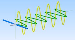
But EM waves tend to organize themselves as they travel away from the antenna and form a perfect match. At a distance of a few wavelengths from the antenna, the electric and magnetic fields coalesce in what’s known as the far-field zone.

Of course, a dipole radiates in all directions perpendicular to its length while we show only one of the traveling directions. As is customary, the balance of this article will consider only the electric waves and their polarizations.

About Linear Polarizations

Using a horizontal and vertical dipole makes it possible to create a composite polarization.

Figure 2 shows how the feed of this combination can change the resulting polarization. In the two images left of center, only one dipole gets a signal. The two images on the right show the dipoles fed in phase and in anti-phase. The result is a slanted polarization. It’s not possible to create a dual polarization at the same time—the fields of the two dipoles will combine into a single EM wave.

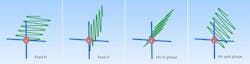
These are all linear polarizations, the EM wave uses only one spatial axis to vibrate. This axis can be horizontal, vertical, or anything in between, depending on how the antenna is oriented.

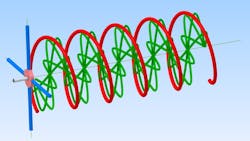
About Circular Polarization

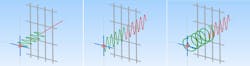
As shown above, connecting the two dipoles in parallel creates a slanted, linear polarization. But if we use a phase-shifting network to feed the second dipole, the straight, slanted line becomes an ellipsis. At a phase shift of 90°, the polarization becomes circular.

Figure 3 shows the two dipoles with different phase shifts from the feed. At 0°, the dipoles produce the slanted polarization. But with a shift of 90°, the EM field becomes circular. Moving on to 180° produces the other slanted orientation, and at 270° (-90°) the EM field becomes circular again, but with an opposite spin.

These two circular polarizations are considered opposite to each other. They’re called left-hand circular polarization (LHCP) and right-hand circular polarization (RHCP).

However, there’s some confusion about these designations. Depending on whether you look out of the antenna (toward the receiver) or at the antenna from the receiver, left becomes right and vice versa.

With antennas and RF EM waves, the convention is to look out from the transmitting antenna to determine whether it’s right- or left-handed. In the optical world, which has the same polarization phenomena with light waves, the definition is the opposite. Fortunately, the RF and the optical worlds are not (yet) crossing paths because of the large frequency difference.

What is the Axial Ratio?

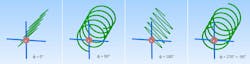
A circular polarized signal can have several deviations from a perfect circular signal. It can have an imbalance between the horizontal and vertical components, or it can have a deviation from +90° or −90° phase shift, or both.

Figure 4 shows what the polarization looks like with unbalanced horizontal and vertical components. It’s assumed that the components have a 90° phase shift.

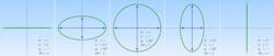
The image on the left has only a horizontal component, so it’s linear and horizontal. In the second image from left, we see polarization in which the vertical component is half the horizontal component, making for an elliptical signal. In the center is a proper circular signal. The two right-side figures have half or zero horizontal components.

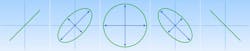
Figure 5 depicts what the signals look like when the phase shift goes from 0° to 180°. At 0° and 180°, we have a linear polarization. At ±45°, the signal is a slanted ellipse, and at 90°, it’s again a proper circular signal.

These deviations can be expressed as the axial ratio (AR), which is the ratio between the two axes of the ellipse. The AR of a perfect circular signal is 1 (1:1), or 0 dB. For imperfect signals, the AR is higher and for a linear polarization it goes to infinite.

The effects of these deviations result in a reduced reception and a limited suppression of the opposite polarization. Although the AR doesn’t describe exactly how the polarization is non-circular, it correlates directly to the attenuation of cross-polarized signals.

About Co- and Cross-Polarization

When both transmitting and receiving antennas have the same polarization, they have co-polarization. The receiver has optimal reception of the transmitted signal.

When an antenna is subject to a polarization opposite of its own polarization, it should not receive anything. But real-world antennas are imperfect and an antenna may still be sensitive to some of the opposite polarization. This is called cross-polarization (XP).

Cross-polarization applies to both linear and circular polarization. A vertical antenna receives little or none of a horizontal signal. Similarly, an RHCP antenna receives little or none of an LHCP signal.

The suppression of cross-polarized signals can be used to attenuate unwanted interfering signals or reflections. For some applications it is an important characteristic.

Calculating Cross-Polarization from Axial Ratio

For circular antennas, the cross-polarization XP can be calculated when the axial ratio is known:

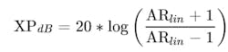
where  is a linear number.

To convert AR from dB to linear:

Mixing Linear and Circular Polarizations

While cross-polarized antennas don’t receive each other, one may wonder how a linear antenna responds to a circular signal and vice versa.

As we have seen before, a circular signal consists of a horizontal and vertical component. Consequently, a linear antenna will always receive a circular signal. No matter how the linear antenna is positioned, it will “see” the circle of the polarization. Likewise, a circular antenna can receive any type of linear polarization because it’s “looking” with its circle.

In these situations, the receiving antenna will only receive half of the signal, so the effective antenna gain is reduced by 3 dB.

Signal Propagation of Different Polarizations

Both linear and circular polarizations have different behavior in environments with (multiple) reflections, such as domestic and urban settings.

Penetration

Most buildings are constructed from concrete containing steel rebar. The concrete itself does have some attenuation, but it’s not dramatic. The rebar, however, can be a large EM obstacle, depending on its spacing and the wavelength involved.

Figure 6 depicts signals traveling through the rebar of a concrete wall. In this example, the rebar is horizontally spaced at a distance smaller than a half-wavelength, while the vertical spacing is larger than that. The rebar forms a kind of filter: Horizontal waves don’t pass through while vertical waves fit through the holes.

For circular waves, the effect is that the horizontal component is stripped off and the resulting wave has a linear, vertical polarization.

Reflection

When a signal reflects from a surface, the polarization components can change depending on the angle and orientation of the surface. Figure 7 shows that the component in-line with the surface is reflected well, while a perpendicular component gets mostly attenuated. In the case of a circular signal, only the in-line component survives and the signal becomes (more) linear.

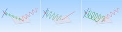
Note that the images in Figure 7 are exaggerated: The amount of surviving signal components depends on the surface and the incidence angle. So, in an urban or domestic environment, circular polarization has a better chance that some of its components will survive the various obstacles, when compared to linear.

On a side note, the polarizing effect of reflection is exploited by Polaroid sunglasses. Because most of the light reflected from the ground or a water surface has mostly horizontal components, it can easily be filtered out by a vertically polarized filter.

Comparison of Linear vs. Circular Applications

Linear and circular polarization have their own application areas because of their propagation difference and antenna designs. The table shows the main aspects and the differences. In general, circular polarization shines in mobile communications while linear polarization best suits fixed communication links.

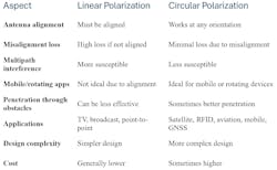
However, linear antennas are typically easier and cheaper to manufacture and can be made more compact than circular antennas. It’s also more difficult to make an omnidirectional circular antenna. Domestic applications often require omnidirectional radiation patterns because the wireless clients are moving around.

For these reasons, many of the small and tiny wireless devices in the market have linear antennas. However, GNSS (GPS) antennas are often circular to match the satellite signals.

Analyzing Circular Polarization

Since we can use two linear antennas to produce circular polarization, it’s also possible to receive a signal with two linear antennas and analyze the polarization properties. By measuring the amplitude of the two signals, we can determine if it’s a horizontal or vertical signal, or something in between.

But the amplitude alone doesn’t tell us if it’s a slanted linear or circular polarization. We also need to measure the phase between the two signals to determine if it’s linear (0° or 180°), circular (±90°), or anything in between.

Many antenna measurement setups aren’t suited for this analysis because they measure one polarity at a time, which makes it impossible to measure the phase between them.

Measuring Linear and Circular Polarizations

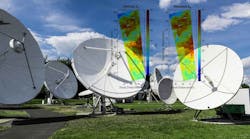
One device that’s suitable for these measurements and subsequent analysis is MegiQ’s Radiation Measurement System (RMS) (Fig. 8). The standalone system, which includes a turntable, dual-polarization antenna and dual-channel, phase-coherent receiver, can measure radiation patterns of standalone wireless devices that transmit a constant carrier or constant test pattern.

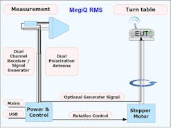
With its built-in tracking generator, the RMS can also perform rotation and sweep measurements of bare antennas. Meanwhile, its phase-coherent receiver allows measurement of the phase between the horizontal and vertical signals and thus calculates the circular properties of an antenna. The system is designed so that only minimal anechoic measures are required to get accurate and meaningful measurements. Figure 9 shows the RMS antenna and turntable; the receiver is mounted behind the antenna.

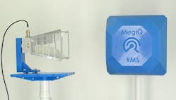
The RMS systems can measure between 370 MHz and 6 GHz, depending on the model. They’re very useful when resources are limited, such as budget and space, and one needs quick antenna measurements and not have to wait and pay for measuring time at a test lab. The accuracy of the RMS is of the same order as certified test labs.

Measurements of a Circular Satellite Communication Antenna

The RMS system measures the horizontal and vertical polarization and their phase relation, and the user can open a graph for linear polarizations or circular polarizations. These graphs use the same measurement, but they differ in the kind of post-processing of the data.

The left-hand graph of Figure 10 shows the linear result. The antenna has roughly equal horizontal (purple) and vertical (brown) components. In the statistics at the bottom line, the maximum of the combined gain is 2.3 dB.

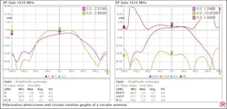
The same maximum of the total gain of 2.3 dB can be found in the right-hand graph, where the gain is converted to a RHCP component (purple) and a LHCP component (brown). Now, there’s a large difference of 17.1 dB between RHCP and LHCP.

The axial ratio (red) is 2.44 dB at the center, which converts to 17.1 dB of cross-polarization.

The rotation radiation patterns in Figure 11 are measured with the same antenna. The graph at left shows how the axial ratio is only good in the main lobe of the antenna and deteriorates to higher values in the other direction.

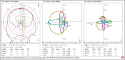
The graphs at center and right show the RHCP and LHCP radiation patterns. Again, a large difference exists between the RHCP and LHCP gains.

Also, the total isotropic gain (TIG), which translates to antenna efficiency of the two components, is very different at −2.9 dB / 51% for RHCP versus −15.4 dB / 2.9% for LHCP.

Measurement of a Circular GNSS Patch Antenna

The frequency sweep in Figure 12 illustrates the linear and circular plots of a GNSS (GPS) patch antenna. In the operational bands, the horizontal and vertical gains are again similar to each other.

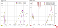
The RHCP and LHCP graphs on the right shows the circular operation of the antenna. The cross-polarization in the main band is around −13 dB. The axial ratio also drops to reasonable levels in the two bands.

In conclusion, linear and circular polarization have their own areas of application. But because it’s more difficult and/or expensive to create very compact circular antennas, they’re not used in some areas that would benefit from it.

Measuring and analyzing circular signals requires a measurement system that can measure the horizontal and vertical components and the phase between them. The MegiQ RMS system is one of the few systems that can do this with good accuracy.