Algorithms to Antenna: Labeling Radar and Comms Signals for Deep-Learning Apps

As part of this series, we have written multiple posts on applying deep-learning techniques to radar and communications applications. The most recent posts related to this topic include:
- Train Deep-Learning Networks with Synthesized Radar and Communications Signals
- RF Fingerprinting for Trusted Communications Link
- Develop and Test Algorithms on Commercial Radars
In these blogs, we synthesized radar and communications data to train deep-learning networks in target and signal classification applications and, most recently, RF fingerprinting. We showed multiple examples where networks were trained with synthesized data and tested the networks with data collected from a radio or radar.
While previous blogs focused on data synthesis, here we look at labeling real-world data from a radar, a radio, or instrumentation. This type of data typically is in a complex format, with an I (in-phase) and Q (quadrature) component. The data is usually contained in sets of large files where the only identifier is in the file name, which might include information on when the data was collected.
Your data can be labeled in many ways. For example, you may label an entire signal by its waveform modulation type. In other applications, labels may indicate what type of target return (aircraft, drone, etc.) or interference is included in the signal. These types of labels are referred to as categorical labels.
Moving to a more granular level, you may label specific characteristics of your signals, such as pulse width, bandwidth, or pulse repetition frequency (PRF). In other applications, labels might indicate regions of interest (ROI); for example, a spurious interference event that occurs at a finite time interval within a larger signal.
We will demonstrate how you can label the primary time and frequency features of pulse radar signals using three common waveforms: linear FM, rectangular, and stepped FM. The workflow helps you to create complete and accurate data sets to train models used for deep learning. Note, this type of workflow can be similarly applied to communications signals as well.
We will start with an interactive tool that was designed for this type of application—the Signal Labeler app—which is part of the Signal Processing Toolbox for MATLAB. For completeness, we will discuss ways to label data manually and automatically using the app.
In manual mode, we leverage synchronized time and time-frequency views to help identify frequency features related to the waveform modulation type. In automated mode, we use functions that identify waveform characteristics, including PRF, pulse width, duty cycle, and pulse bandwidth.
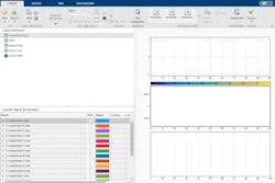
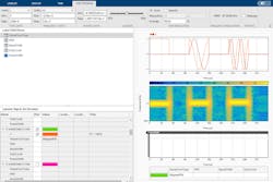
Figure 1 shows the Signal Labeler app with radar signals loaded and ready to be labeled. There’s a Label Definitions panel (top left) and panels for the key visualizations (right). To start, we create a label definition for each of our signal waveform types. For our example, these label values are LinearFM, Rectangular, and SteppedFM. As part of our setup, we also create attribute label definitions for PRF, duty cycle, pulse width, and bandwidth. These parameters will be automatically labeled using functions that process each signal.
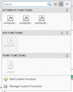
We use an ROI label to capture a region in each signal that spans from the initial and final times over which an event or characteristic of interest occurs for the characteristic we want to label. Once the labels are defined, you can upload custom functions you author in MATLAB to the labeler. For our example, we use functions customized to label the PRF, bandwidth, duty cycle, and pulse width. Figure 2 shows a zoomed view of the automated functions gallery in the labeler toolstrip.
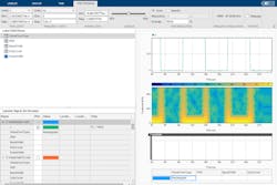
As we noted earlier, to demonstrate the ability to manually label a signal, we first inspect the signal in the time and time-frequency domains (Fig. 3). Once we visually determine the signal type by looking at the time-frequency content, we can manually assign the label. A few notes to keep in mind: The signals we use in the example are ideal signals to make it easy to see the attributes; however, these same techniques can be used effectively on noisy signals with any number of impairments. In addition, labeling can be done automatically by applying the techniques described below.
Note that the waveform characteristics aren’t filled in yet (Fig. 3, bottom right). We will show how to do this labeling shortly. For the manual labeling portion of the workflow, the labels you define (in this case, the waveform types) are available in the dropdown menu, which you can pick from.
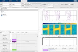
Figures 4 and 5 show the similar visualizations for the linear FM and stepped FM waveforms, respectively. Note the respective waveform type label has been added for each signal.
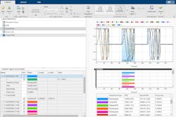
With the manual labeling complete for each waveform type, we can now use functions to automatically compute and label the characteristics of each input signal. For more information on the functions used in our example, and how you can add and customize your own functions, please go here. The results are shown in the bottom-right section of Figure 6. The nice part of this workflow is that you can customize your own functions in MATLAB and add them to the function gallery in the Signal Labeler app.
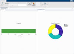
We have a small data set in this example, but you would typically have much larger sets. You can view your labeling progress and verify the computed label values are correct. Figure 7 (left) shows the labeling progress, which in this example is 100%, as all signals are labeled. Figure 7 (right) shows the number of signals with labels for each label value. The pie chart can be utilized to ensure you have a balanced data set. In this case, you can also assess the accuracy of your labeling and confirm the results are as expected.
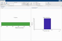
Furthermore, the dashboard can be used to analyze signal region labels. For example, we can see in Figure 8 that all pulse-width label values are distributed around 5e-5, which matches our data-set ground truth.
When labeling is completed, you can export the labeled signals back into MATLAB to train your deep-learning models.
To learn more about the topics covered in this blog and explore your own designs, see the examples below or email me at [email protected]:
- Automatically Label Radar Signals (example): Learn how to label the main time and frequency features of pulse radar signals and create complete and accurate data sets to train artificial-intelligence (AI) models.
- AI for Radar (examples): Learn how AI techniques can be applied to radar applications.
- Deep Learning in Wireless Systems (examples): Learn how deep-learning techniques can be applied to wireless applications.
See additional 5G, radar, and EW resources, including those referenced in previous blog posts.
Rick Gentile is Product Manager, Shrey Joshi is Senior Engineer, Frantz Bouchereau is Engineering Manager, and Honglei Chen is Principal Engineer at MathWorks.
About the Author
Rick Gentile
Product Manager, Phased Array System Toolbox and Signal Processing Toolbox
Rick Gentile is the product manager for Phased Array System Toolbox and Signal Processing Toolbox at MathWorks. Prior to joining MathWorks, Rick was a radar systems engineer at MITRE and MIT Lincoln Laboratory, where he worked on the development of several large radar systems. Rick also was a DSP applications engineer at Analog Devices, where he led embedded processor and system level architecture definitions for high performance signal processing systems used in a wide range of applications.
He received a BS in electrical and computer engineering from the University of Massachusetts, Amherst, and an MS in electrical and computer engineering from Northeastern University, where his focus areas of study included microwave engineering, communications, and signal processing.
