Algorithms to Antenna: Modeling Air-Traffic-Control Radar Systems
In this latest edition of Algorithms to Antenna, we build on the examples described in our previous blog, where we modeled a radar network to track space debris. As we highlighted in the space debris example, you can model radars to improve your system-level knowledge and ensure design choices are sound before you acquire or build them. For the examples described in this blog, we use a set of air-traffic-control examples to extend our discussion in two directions. The first involves fusing information from another sensor modality to improve the overall system-level performance. The second focuses on providing easy ways to generate larger data sets to help make system architecture decisions and provide more robust system-level testing.
To set the stage, we start with a little background. The Federal Aviation Administration (FAA) is responsible for the regulation of flights across United States airspace. The air-traffic-control system is a complex, multilevel system. Air-traffic towers monitor and handle flights in the immediate vicinity of an airport, while Air Route Traffic Control Centers (ARTCCs) are responsible for long-range surveillance.
The capabilities and corresponding levels of complexity of air-traffic/surveillance radars have increased significantly over the past decades. The addition of transponders on aircraft provides a communication link to the air-traffic facilities, which increases accuracy of positioning estimates. This benefits decision-making at the control centers.
Today, aircraft flying above 10,000 feet must be equipped with an Automatic Dependent Surveillance Broadcast (ADS-B) transponder to broadcast their estimated position. The Navigation Accuracy Categories used in ADS-B systems for position and velocity are referred to as NACp and NACv, respectively. NACp specifies the accuracy of an aircraft’s horizontal position information (latitude and longitude). NACv is an estimate of the accuracy of the horizontal geometric velocity output. Based on FAA regulations, the accuracy for NACp must be within 0.05 nautical miles and the NACv accuracy must be within 10 meters per second.
Air Route Surveillance Radar 4 (ARSR-4) is one type of long-range surveillance radar used by the FAA. It provides 3D returns at ranges up to 250 nautical miles (463 kilometers). Most ARSR-4 radars are located along the borders of the continental United States, while slightly shorter-range radars are mostly located at FAA radar sites. In our first example, we use a collection of three ARSR-4 radar sites, each with the following technical specifications:
- Update rate: 12 sec
- Maximum range (1 meter-square target): 463 km
- Range resolution: 323 m
- Range accuracy: 116 m
- Azimuth field of view: 360 deg
- Azimuth resolution: 1.4 deg
- Azimuth accuracy: 0.176 deg
- Elevation accuracy: 900 m
For simplicity, we start with a single flight trajectory that spans thousands of kilometers between two airports. We use sensor models to generate synthetic detections of the aircraft as seen by three radars. Radar detections are fused centrally to maintain situational awareness as the aircraft moves along its route.
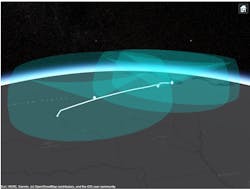
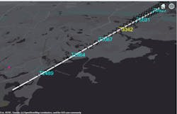
In the first simulation, only the three radars are used to track the aircraft. In Figure 1, each of the three radar locations is indicated by a diamond. The coverage for each radar is also visualized in Figure 1. The white line represents the trajectory of the aircraft in the simulation.
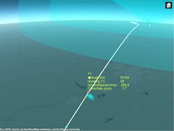
In Figure 2, you can see the results of the first leg of the flight. The detections have high measurement noise because the aircraft is in the outer regions of radar coverage. The large ellipsoids around the detections in Figure 2 (left) represent the higher uncertainty in the measurements. As the aircraft enters the coverage area of the second surveillance radar, additional detections with less uncertainty help to correct the track shown in Figure 2 (right). The track (in yellow) follows the truth (in white) much closer as it enters the coverage area of the second radar.
Fusing Additional Positioning Information
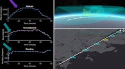
To improve the accuracy of the fused radar-detection results, we now fuse ADS-B positioning data to improve the overall tracking quality. In Figure 3, ADS-B detections are represented in purple.
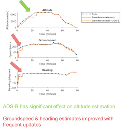
In Figure 4, the results show that the additional data provided by ADS-B significantly affects the altitude estimation, which is the least accurate information reported by the radars. In addition, the groundspeed and heading estimates are improved with the benefit of more frequent updates. The radars in our simulation provide updates every 12 seconds, while the ADS-B reports come in every second.
This type of modeling can be extended to other applications that use additional sensor modalities (e.g., LiDAR, vision, and EO/IR) and positioning systems (e.g., AIS, TDOA, and FDOA). The sensor parameters can be adjusted to match specific sensor parameters. Sensor locations, update rates, and tracking architectures can be modified based on the application, too.
Increasing System Testing
It’s also possible to improve system testing with system-level modeling. The ability to generate test data for large, complex systems is invaluable. This additional data can help you understand what to expect in field tests. In addition, it may help in system-level debug when unexpected results are measured in the field. On top of that, such data generation can train deep-learning networks to recognize anomalous conditions in your systems.
Continuing with the air-traffic-control theme, we now look at ways to automatically detect deviations and anomalies in aircraft making final approaches to an airport runway. To start, we model an ideal landing approach trajectory as shown in Figure 5 (left). From the ideal landing, we can programmatically generate variants from it.
An aircraft in final approach to landing must align itself with the runway, gradually descend to the ground, and reduce its ground speed while keeping it safely above stall speed. All of these steps are taken to ensure that the aircraft touches the ground softly to reduce the risk to passengers and avoid physical damage to the aircraft or the runway. These rules are easily set by an aviation professional and in this example, we use rules previously defined. For our initial trajectory, we define “safe” to be as follows:
- The trajectory must be closely aligned with the runway direction.
- The glide slope must be between 2.5 and 4 degrees in the last 20,963 meters.
- At distances above 20,963 meters, the altitude must be at least 3000 ft.
- The speed must be between 120 and 180 knots at the landing point.
- The upper speed bound can increase linearly with distance from the landing point.
To generate additional trajectories, we perturb each waypoint in the trajectory with a zero-mean normal distribution and a standard deviation that gets smaller from the first waypoint to the last (the landing point). At the first waypoint, the standard deviation is 5e-3 degrees in longitude and 300 meters in altitude. The standard deviation decreases to 1e-3 degrees in longitude and 150 meters in altitude in the midpoint, and then to 1e-4 degrees in longitude and 0 in altitude at the end-point on the ground.
Aircraft approaching landing are scheduled to avoid the aerodynamic impact from one aircraft on the aircraft following in its wake. The minimum safe time difference between two aircraft is one minute. We schedule the trajectories generated earlier by adding random perturbations to the time of arrival at each waypoint with about a minute of separation between the landing aircraft.
In Figure 5 (right), we plot the trajectories in yellow for anomalous trajectories and cyan for safe approaches.
Detecting anomalies in real time based on tracking data is a challenge for several reasons. First, since the tracking data is imperfect with noise, the tracking results are uncertain. As a result, some tolerances must be provided to avoid issuing false warnings. Second, the sensors report false detections, and the tracking system must be careful not to confirm tracks based on them.
In Figure 6, tracks that violate the safe approach rules are shown in yellow, while tracks that follow these rules are shown in cyan. Note that the warning is issued immediately when the track violates any rule, and it’s removed when satisfying all of the rules.
This type of data generation can be extended to match different radar configurations. Other system parameters are able to be adjusted to match your application. With these data types in place, you can build more robust system-level architectures and feel more confident in system design choices before systems are modified or designed.
To learn more about the topics covered in this blog, see the examples below or email me at [email protected]:
- Simulate and Track En-Route Aircraft in Earth-Centered Scenarios (Example): Learn how to use two different models to generate synthetic detections of the airplane: a monostatic radar and ADS-B reports. Learn to use a multi-object tracker to estimate the plane trajectory, compare the tracking performance, and explore the impact that ADS-B provides on the overall tracking quality.
- Simulate, Detect, and Track Anomalies in a Landing Approach (Example): Learn how to detect deviations and anomalies in aircraft making final approaches to an airport runway.
- Air Traffic Control System Modeling (Example): Learn how to simulate a multifunction phased-array radar system.
See additional 5G, radar, and EW resources, including those referenced in previous blog posts.
Rick Gentile is Product Manager, Gael Goron is a Software Engineer, Elad Kivelevitch is Senior Team Lead, and Honglei Chen is Principal Engineer at MathWorks.
