Algorithms to Antenna: Tracking Space Debris with a Radar Network
In past blogs, we have discussed a range of radar modeling examples, including a multifunction radar and multistatic systems. Here, we show how to model a network of radar systems that look into space with the mission of tracking debris orbiting Earth. These types of models can aid in radar system design, but they can also help with system-level tradeoffs in terms of how many radars are needed, where each radar is located, how well each radar has to perform, and how much data must be transferred between each sensor. Such information helps drive system architecture decisions.
First, a bit of background on the model we will discuss. Unfortunately, the amount of space debris in Earth’s orbit has increased substantially and continues to do so at an accelerated pace. The European Space Agency estimates more than 30,000 large debris objects (diameter >10cm) and more than 1 million smaller debris objects are in low Earth orbit (LEO).
This debris presents a danger to human activities in space. For example, the debris could damage operational satellites and force time-sensitive and costly avoidance maneuvers of space-based assets. As space activity increases, keeping track of space debris becomes ever-more crucial.
Our model starts with a scenario we will use as a test bench for our system. Earth-centric trajectories are generated to set space debris in motion around the earth. The debris trajectories are used to drive a scenario that generates synthetic radar detections of this debris. Our goal is to use these detections to obtain and track position and velocity estimates for each object.
Trajectories of space objects rotating around Earth can be approximated with a Keplerian model, which assumes that Earth is a point-mass body and the objects orbiting around it have negligible masses. This example doesn’t account for higher-order effects in Earth’s gravitational field and environmental disturbances, but they could easily be added. The equation of motion is expressed in an Earth-centered, Earth-fixed (ECEF) frame. Since this is a non-inertial reference frame, it accounts for the Coriolis and centripetal forces.
First, we create initial positions and velocities for the space-debris objects. This is done by obtaining the traditional orbital elements (semi-major axis, eccentricity, inclination, longitude of the ascending node, argument of periapsis, and true anomaly angles) of these objects from random distributions. These orbital elements are converted to position and velocity vectors.
For our example, we define four antipodal radar stations that provide fan-shaped beams looking into space. Each radar’s coverage cuts through the orbits of debris objects to maximize the number of object detections. Our hypothetical radar locations include one in the Pacific Ocean, one in the Atlantic Ocean, and one near each of the poles.
Having four radars at different locations enables the detection of space debris at points where the additional measurements can be used to correct their position estimates. These locations help in the acquisition of new debris detections.
Each site is equipped with a radar modeled statistically based on the radar equation. The statistical radar models provide the fastest way to generate detections. However, as we previously blogged about in the multifunction radar example, these types of radars can also be modeled to generate I/Q signals that consider areas like the phased-array antenna design, signal processing, and environmental conditions. For ease of discussion, we will stick to the statistical model here. With this, we can define the main requirements for our radar.
To detect debris objects in the LEO range, the radar has the following requirements:
- Detect a 10-dBsm object up to 2000 km away.
- Resolve objects horizontally and vertically with a precision of 100 m at 2000-km range.
- Cover a field of view of 120 degrees in azimuth and 30 degrees in elevation.
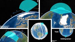
Figure 1 shows a virtual globe with all of the modeling elements defined in the scenario, including individual debris in their trajectories, radar coverage beams, radar detections, and radar tracks.
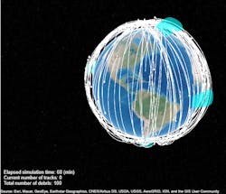
On the virtual globe, space debris is represented by white dots with individual trailing trajectories shown by white lines. Most of the generated debris objects are on orbits with high inclination angles close to 80 degrees. The trajectories are plotted in ECEF coordinates; therefore, the entire trajectory rotates toward the west due to Earth’s rotation. After several orbit periods, all space debris passes through the surveillance beams of the radars.
A multi-object tracker is used to create new tracks, associate detections with existing tracks, estimate their state, and delete divergent tracks. The tracker receives information as to whether a tracked object is detectable in the surveillance region. This is important so as to not penalize tracks that are propagated outside of the radar surveillance areas.
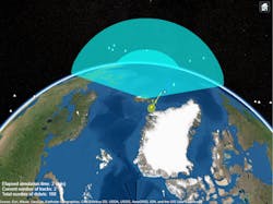
In Figure 2, you can see an object being tracked as track T1 in yellow. This object was detected only twice, which wasn’t often enough to reduce the uncertainty of the track. Therefore, the size of its covariance ellipse is relatively large.
In Figure 3, you can observe another track T2 in blue, which is detected by the sensor several times. Its corresponding covariance ellipse is much smaller since more detections were used to correct the state estimate.

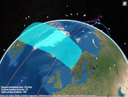
In Figure 4, track T12 (in purple) is about to enter the radar surveillance area. Track T10 (in orange) was just updated with a detection, which reduced the uncertainty of its estimated position and velocity.
Different radar station locations and configurations could be explored to increase the number of tracked objects. You can also gain insights into how changes in radar specifications can impact the overall system-level performance.
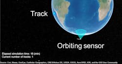
Before concluding, we want to show you a variant of the first example that we’re often asked about. Here, instead of ground-based radars, we can use the same radar model on a moving platform. Figure 5 shows the results where the radar is looking downward. Here, the target is on the ground and is tracked from the radar orbiting from above.
To learn more about the topics covered in this blog, see the examples below or email me at [email protected].
- Track Space Debris Using a Keplerian Motion Model (Example): Learn how to model Earth-centric trajectories using custom motion models, configure a monostatic radar sensor to generate synthetic detections of space debris, and set up a multi-object tracker to track the simulated targets.
- Search and Track Scheduling for Multifunction Phased Array Radar (Example): Learn how to simulate a multifunction phased-array radar system.
- Multiplatform Radar Detection Generation (Documentation): Learn how to generate radar detections from a multiplatform radar network.
See additional 5G, radar, and EW resources, including those referenced in previous blog posts.
Rick Gentile is Product Manager, Gael Goron is a Software Engineer, Elad Kivelevitch is Senior Team Lead, and Honglei Chen is Principal Engineer at MathWorks.
About the Author
Rick Gentile
Product Manager, Phased Array System Toolbox and Signal Processing Toolbox
Rick Gentile is the product manager for Phased Array System Toolbox and Signal Processing Toolbox at MathWorks. Prior to joining MathWorks, Rick was a radar systems engineer at MITRE and MIT Lincoln Laboratory, where he worked on the development of several large radar systems. Rick also was a DSP applications engineer at Analog Devices, where he led embedded processor and system level architecture definitions for high performance signal processing systems used in a wide range of applications.
He received a BS in electrical and computer engineering from the University of Massachusetts, Amherst, and an MS in electrical and computer engineering from Northeastern University, where his focus areas of study included microwave engineering, communications, and signal processing.
