Phased-Array Antenna Patterns (Part 1)—Linear-Array Beam Characteristics and Array Factor
>> Microwaves & RF Resources
.. >> Library: Article Series
.. .. >> Topic: Phased-Array Antenna Design
.. ... .. >> Phased-Array Antenna Patterns
Download this article in PDF format.
With the proliferation of digital phased arrays in commercial as well as aerospace and defense applications, there are many engineers working on various aspects of the design who have limited familiarity with phased-array antennas. Phased-array antenna design isn’t new, as the theory has been well developed over decades. Most of the literature, though, is intended for antenna engineers who are proficient with the electromagnetic mathematics.
However, as phased arrays begin to include more mixed-signal and digital content, many engineers could benefit from a much more intuitive explanation of phased-array antenna patterns. As it turns out, many analogies exist between the behavior of phased-array antennas and the discrete time-sampled systems that the mixed-signal and digital engineers work with every day.
Beam Direction
First, let’s look at an intuitive example of steering a phased-array beam. Figure 1 provides a simple illustration of a wavefront striking four antenna elements from two different directions. A time delay is applied in the receive path after each antenna element, and then all four signals are summed together. In Figure 1a, that time delay matches the time difference of the wavefront striking each element. And in this case, that applied delay causes the four signals to arrive in phase at the point of combination. This coherent combining results in a larger signal at the output of the combiner.
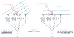
In Figure 1b, that same delay is applied. But in this case, the wavefront is perpendicular to the antenna elements. That applied delay now misaligns the phase of the four signals, significantly reducing the output of the combiner.
In a phased array, time delay is the quantifiable delta needed for beamsteering. But time delay can also be emulated with a phase shift, which is common and practical in many implementations. We will discuss the impact of time delay vs. phase shift in the section on beam squint. For now, though, let’s look at a phase-shift implementation, and then derive the calculation for beamsteering with that phase shift.
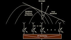
Figure 2 shows this phased-array arrangement using phase shifters rather than time delay. Note that we define the boresight direction (θ = 0°) as perpendicular to the face of the antenna. A positive angle θ is defined to the right of boresight, and a negative angle is defined to the left of boresight.
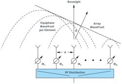
To visualize the phase shift needed for beamsteering, a set of right triangles can be drawn between adjacent elements (Fig. 3), where ΔΦ is the phase shift between those adjacent elements.
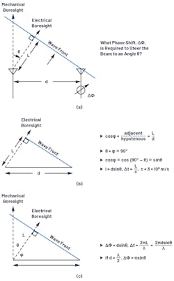
Figure 3a defines the trigonometry between those elements, with each element separated by a distance (d). The beam is pointed in a direction off boresight, θ, which is an angle, φ, from the horizon. In Figure 3b, we see that the sum of θ + φ = 90°. This allows us to compute L, the delta distance of wave propagation, as L = dsin(θ). The time delay to steer our beam is equal to the time it will take for the wavefront to traverse that distance, L.
If we think of L as a fraction of the wavelength, then a phase delay could be substituted for that time delay. The equations for ΔΦ can thus be defined relative to θ, as shown in Figure 3c, and repeated in Equation 1:

If the spacing between elements is exactly one half of the signal wavelength, then this can further be simplified to:

Let’s work out an example with these equations. Consider two antenna elements spaced 15 mm apart. If a 10.6-GHz wavefront is arriving at 30º from mechanical boresight, then what’s the optimal phase shift between the two elements?
- θ = 30º = 0.52 rad
- λ = c/f = (3 × 10⁸ m/s)/10.6 GHz = 0.0283 m
- ∆Φ = (2π × d × sinθ)/λ = 2π × 0.015 × sin(0.52)/0.0283 m = 1.67 rad = 95º
So, if our wavefront is arriving at θ = 30º, and we then shift the phase of the neighboring element by 95º, we will cause the individual signals of both elements to add coherently. This will maximize the antenna gain in that direction.
For a better appreciation of how the phase shift varies with the beam direction (θ), these equations are plotted for a variety of conditions in Figure 4. Some interesting observations can be made from these graphs.
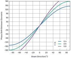
For the case of d = λ/2, there’s an approximate 3 to 1 slope near boresight, which is the π multiplier in Equation 2. This case also shows a full 180° shift between elements, which provides a theoretical 90° shift in beam direction. In practice (with real element patterns), this isn’t realizable; yet, the equations do show the theoretical ideal. Note that for d > λ/2, no amount of phase shift provides a full beam shift. Later, we will see that this case can lead to grating lobes in the antenna pattern, and this graph provides a first indicator that something is different with the d > λ/2 case.
A Uniformly Spaced Linear Array
The equations developed above have applied to just two elements. Yet, a real phased array can be thousands of elements spaced across two dimensions. But for now, let’s just consider one dimension: a linear array.
A linear array is a single element wide with N number of elements across. The spacing may vary, but often it’s uniform. Therefore, for purposes of this article, we will set the spacing between each element to a uniform distance, d (Fig. 5). Although simplified, this uniformly spaced linear-array model provides the foundation for insight into how the antenna pattern is formed in light of various conditions. We can further apply the principles of the linear array to understand two-dimensional arrays.

Near Field vs. Far Field
So how can we take the equations previously developed for an N = 2 linear array and apply them to an N = 10,000 linear array? Right now, it seems that each antenna element has a slightly different angle pointing to the spherical wavefront (Fig. 6).
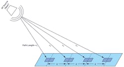
With the RF source near, the incident angle varies for each element. This situation is called the near field. We can work out all of these angles, and sometimes we need to do this for antenna testing and calibration as our test setup can only be so large.
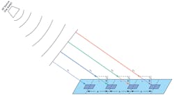
But if we assume that the RF source is far away (Fig. 7), the large radius of the spherical wavefront results in wave propagation paths that are approximately parallel. Therefore, all of our beam angles are equal, and each adjacent element has a path length that is L = d × sinθ longer than its neighbor. This simplifies the math and means that the two-element equations we derived earlier can be applied to thousands of elements, provided they have uniform spacing.
But when can we make the far-field assumption? How far is far? It’s a little subjective, but in general, far field is considered anything greater than:

where D is the diameter of the antenna ((N-1) × d for our uniform linear array).
For a small array (small D) or a low frequency (large λ), the far-field distance is small. But for a large array (or high frequency), the far-field distance could be many kilometers. That makes it hard to test and calibrate the array. For such conditions, a more-detailed near model may be used, and then bridge this back to the far-field, real-world use of the array.
In Part 2, we’ll cover antenna gain, directivity, and aperture, as well as array factors.
Authors’ Note: This series of articles is not intended to create antenna design engineers, but rather to help the engineer working on a subsystem or component used in a phased array to visualize how their effort may impact a phased-array antenna pattern.
Peter Delos is Technical Lead and Bob Broughton is Director of Engineering for Analog Devices' Aerospace and Defense Group, and Jon Kraft is Senior Staff Field Applications Engineer at Analog Devices.
References
Balanis, Constantine A. Antenna Theory: Analysis and Design. Third edition, Wiley, 2005.
Mailloux, Robert J. Phased Array Antenna Handbook. Second edition, Artech House, 2005.
O’Donnell, Robert M. “Radar Systems Engineering: Introduction.” IEEE, June 2012.
Skolnik, Merrill. Radar Handbook. Third edition, McGraw-Hill, 2008.
>> Microwaves & RF Resources
.. >> Library: Article Series
.. .. >> Topic: Phased-Array Antenna Design
.. ... .. >> Phased-Array Antenna Patterns
About the Author
Peter Delos
Technical Lead, Aerospace and Defense Group, Analog Devices
Peter Delos is a technical lead in the Aerospace and Defense Group at Analog Devices in Greensboro, N.C. He received his BSEE from Virginia Tech in 1990 and MSEE from NJIT in 2004. Peter has over 25 years of industry experience, with most spent designing advanced RF/analog systems at the architecture level, PWB level, and IC level. He’s currently focused on miniaturizing high-performance receiver, waveform generator, and synthesizer designs for phased-array applications.
