Algorithms to Antenna: Developing Beamformers for Phased-Array Systems
Phased-array systems have many advantages over single antennas. One advantage of having multiple transmit and receive elements is that you can apply complex weighting to each element to form a beam. On transmit, this approach could result in more energy in a specific azimuth and/or elevation, depending on the array geometry. On the receive side, beamformers are designed to strengthen signals coming from desired directions and suppress signals and noise arriving from other directions.
In this blog, we describe some common types of beamforming algorithms. We also describe a framework to develop and test your own beamformers. Note that beamforming isn’t limited to plane waves, but we will only cover these far-field scenarios here.
It’s convenient to think of beamforming in two categories: data independent (conventional) and data dependent (adaptive). Conventional beamforming can be realized with a range of different techniques, such as delay-and-sum beamforming, phase-shift beamforming, subband beamforming, and filter-and-sum beamforming. These beamformers include fixed weights and parameters that don’t depend on the signals at the array. The weights are chosen to produce a specified array response to the signals and interference in the environment.
A signal arriving at an array has different times of arrival at each array element. For example, plane waves arriving at a linear array have a time delay that’s a linear function of distance along the array. Delay-and-sum beamforming compensates for these delays by applying a reverse delay to each sensor so that the signals from each element add constructively. For narrowband signals, time delays can be added with phase shifts in the frequency domain.
For broadband signals, several common approaches are available. One approach is to delay the signal in time by a discrete number of samples. This technique can be tricky because the degree of resolution is determined by the sampling rate of your data. You may not be able to resolve delay differences less than the sampling interval.
A second method involves interpolation of the signal between samples. And a third method uses Fourier transforms on the signals, where a linear phase shift is applied, and then converts the signal back into the time domain. For this approach, phase-shift beamforming is performed at each frequency band.
The advantages of a conventional beamformer are simplicity and ease of implementation. Another advantage is its robustness against steering errors and signal direction errors. A disadvantage is the broad main lobe, which decreases resolution of closely spaced sources or targets. A second disadvantage is that it has large side lobes that allow interference sources to leak into the main beam.
When we discuss data-dependent beamformers, the terms optimal or adaptive beamformers are sometimes used interchangeably, but they’re not quite the same. Optimal beamformers apply weights that are determined by optimizing some quantity. For example, a minimum-variance distortionless-response (MVDR) beamformer determines weights by maximizing the signal-to-noise and interference ratio of the array output. The MVDR beamformer offers several advantages:
- It incorporates noise and interference into an optimal solution.
- It has higher spatial resolution than a conventional beamformer.
- It puts nulls in the direction of interference sources.
- Side-lobe levels are smaller and smoother.
Conversely, an MVDR beamformer is sensitive to errors in either the array parameters or arrival direction. The MVDR beamformer also is susceptible to self-nulling. In addition, trying to use MVDR as an adaptive beamformer requires a matrix inversion every time the noise and interference statistics change. When there are many array elements, the inversion can be computationally expensive to implement.
In practical applications, an accurate steering vector and an accurate covariance matrix aren’t always available. Many times, all that’s available is the sampled covariance matrix. This can lead to both inadequate interference suppression and distortion of the desired signal. That is, if the true signal direction is slightly off from the beam pointing direction, the actual signal is treated as interference.
When noise isn’t separable from the signal, you can estimate a sample covariance matrix from the data. A linear-constraint minimum-variance (LCMV) beamformer is a generalization of MVDR beamforming. Several different approaches can be taken to specify constraints, such as amplitude and derivative constraints. You can, for example, specify weights that suppress interfering signals arriving from a particular direction while passing signals from a different direction without distortion. The advantages and disadvantages of the MVDR beamformer also apply to the LCMV beamformer.
Beamforming Examples
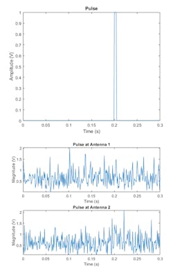
Let’s look at an example in which we apply digital beamforming to a narrowband signal received by an antenna array. For this example, we use the simple rectangular pulse (at baseband) shown in Figure 1. Our signal’s carrier frequency is 100 MHz, and the receiver is a uniform linear array (ULA) with 10 elements spaced by half wavelength. The signal source is 45 degrees of the array boresight. The total return has 10 columns, where each column corresponds to one antenna element. Figure 1 also shows the magnitude plot of the signal for the first two channels in the presence of noise. Note that looking at the pulses before beamforming makes it hard to see the desired signal.
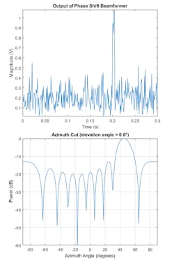
We first use a conventional beamformer to simply delay the received signal at each antenna so that the signals are aligned as if they arrive at same time. In the narrowband case, this is equivalent to multiplying the signal received at each antenna by a phase factor.
In Figure 2, we can see that the signal becomes much stronger compared with the noise. The output signal-to-noise ratio (SNR) is approximately 10 times stronger than that of the received signal on a single antenna because a 10-element array produces an array gain of 10. Figure 2 also shows the pattern of the beamformer. You can see that the main beam of the beamformer is pointing in the desired direction (45 degrees).
In the presence of strong interference, the target signal may be masked by the interference signal. For example, interference from a nearby RF emitter can blind the antenna array in that direction. If the radio signal is strong enough, it may blind the radar in multiple directions, especially when the desired signal is received by a side lobe. These types of scenarios are very challenging for a phase-shift beamformer, which is where adaptive beamformers can help.
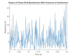
To demonstrate this, we add two interference signals arriving from 30 degrees and 50 degrees in azimuth. Even with low noise levels, interference alone can make a phase-shift beamformer fail. Figure 3 shows the results with the phase-shift beamformer used to retrieve the signal along the incoming direction. You can see that, because the interference signals are stronger than the target signal, we can’t extract the signal content.
To overcome the interference problem, you can use the MVDR beamformer, which is an adaptive beamformer. The MVDR beamformer preserves the signal arriving along a desired direction and tries to suppress signals coming from other directions. In this case, the desired signal is at the direction 45 degrees in azimuth. Figure 4 shows the results using an MVDR beamformer output signal. You can see that the target signal can now be recovered.
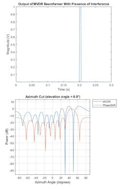
Specifically, Figure 4 shows the response pattern of the beamformer. Note two deep nulls along the interference directions (30 and 50 degrees). The beamformer also has a gain of 0 dB along the target direction of 45 degrees. The MVDR beamformer preserves the target signal and suppresses the interference signals. Also shown is the response pattern from the phase-shift beamformer. The pattern doesn’t null out the interference at all.
This is good to see, but we may not always be able to separate the interference from the target signal. If the target signal is received along a direction slightly different from the desired one, the MVDR beamformer suppresses the desired signal as well. This effect is sometimes referred to as signal self-nulling.
To prevent signal self-nulling, we can use an LCMV beamformer, which allows us to put multiple constraints along the target direction (steering vector). It reduces the chance that the target signal will be suppressed when it arrives at a slightly different angle from the desired direction.
Now we need to create several constraints. First, we preserve the incoming signal from the expected direction (43 degrees). To avoid self-nulling, we ensure that the response of the beamformer will not decline at more than ±2 degrees of the expected direction. We can apply the beamformer to the received signal. Figure 5 shows that the target signal can be detected again even though there’s the mismatch between the desired and the true signal arriving direction.
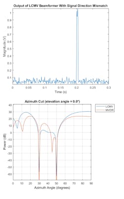
The LCMV response pattern shows that the beamformer puts the constraints along the specified directions while nulling the interference signals along 30 and 50 degrees. The effect of constraints can be better seen when comparing response pattern of the LCMV beamformer with the MVDR beamformer. Notice how the LCMV beamformer is able to maintain a flat response region around the 45 degrees in azimuth, while the MVDR beamformer creates a null.
Comparing Beamformer Performance
You can also use Simulink to set up a test harness and compare beamforming algorithms directly. Let’s keep the last example as the testbench. Again, we have a desired signal we’re trying to recover in the presence of two interference signals arriving from 30 degrees and 50 degrees in azimuth. The interference amplitudes are much larger than the desired signal’s amplitude. Phase shift, MVDR, and LCMV beamformers are applied to the received signal and their results are compared. Figure 6 shows a framework in which you can add your own beamforming algorithms, with controlled inputs to test the corner cases you expect to see in your application.
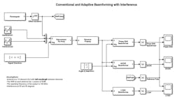
Figure 7 shows the output of the phase-shift beamformer. It’s not able to detect the pulses because the interference signals are much stronger than the pulse signal.
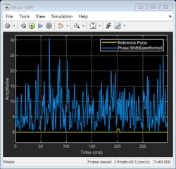
Figure 8 shows the output of the MVDR beamformer. It preserves the signal arriving along a desired direction while trying to suppress signals coming from other directions. In this example, both interference signals were suppressed and the pulse at 45 degrees azimuth was preserved.
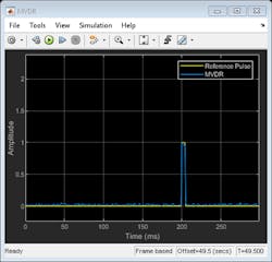
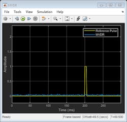
As we noted earlier, the MVDR beamformer is very sensitive to the beamforming direction. If the target signal is received along a direction slightly different from the desired direction, the MVDR beamformer suppresses it. In our Simulink model, you can change the signal direction location to 43 degrees (instead of 45). Figure 9 shows that the received pulses have been suppressed as compared with the reference pulse.
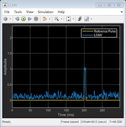
Finally, the LCMV beamformer is used to prevent signal self-nulling by broadening the region surrounding the signal direction where you want to preserve the signal. Figure 10 shows that the desired pulse is preserved.
Beamforming is an important aspect of phased-array systems. As with all engineering challenges, tradeoffs between system performance and computational complexity can be made. You can use system models to help make good decisions before you build your systems.
To learn more about the topics covered in this blog, see the examples below or email me at [email protected]:
- Conventional and Adaptive Beamformers using MATLAB (example): Learn how to apply digital beamforming to a narrowband signal received by an antenna array. Three beamforming algorithms are illustrated: the phase-shift beamformer, the minimum-variance distortionless-response (MVDR) beamformer, and the linear-constraint minimum-variance (LCMV) beamformer.
- Conventional and Adaptive Beamformers using Simulink (example): Learn how to apply conventional and adaptive beamforming in Simulink to a narrowband signal received by an antenna array.
- Beamforming Overview (documentation): Learn how to model narrowband and broadband beamformers.
See additional 5G, radar, and EW resources, including those referenced in previous blog posts.
About the Author
Rick Gentile
Product Manager, Phased Array System Toolbox and Signal Processing Toolbox
Rick Gentile is the product manager for Phased Array System Toolbox and Signal Processing Toolbox at MathWorks. Prior to joining MathWorks, Rick was a radar systems engineer at MITRE and MIT Lincoln Laboratory, where he worked on the development of several large radar systems. Rick also was a DSP applications engineer at Analog Devices, where he led embedded processor and system level architecture definitions for high performance signal processing systems used in a wide range of applications.
He received a BS in electrical and computer engineering from the University of Massachusetts, Amherst, and an MS in electrical and computer engineering from Northeastern University, where his focus areas of study included microwave engineering, communications, and signal processing.
