You Can Now Achieve Zero-Bandwidth Modulation
Series: April 1, 2020: What's Trending in Technology?
The curse of the communications engineer has always been getting maximum data rate through the narrowest channel. In broadband applications, modulation provides the carrier, but in all cases, the resulting sidebands eat up the bandwidth. Now a recent discovery lets you achieve your data objective with zero bandwidth.
Hidden from discovery in plain view for decades, this method has some engineers wondering if all that they ever knew about spectral efficiency is wrong. You can prove this recent discovery by going through the math yourself. All you really need to remember are some basic trigonometric identities:
- sin A sin B = 0.5[cos (A − B) − cos (A + B)]
- cos A cos B = 0.5[cos (A − B) + cos (A + B)]
- sin A cos B = 0.5[sin (A − B) + sin (A + B)]
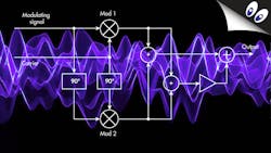
Write the math through the modulation circuit in the figure and voilà…
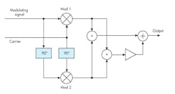
The primary signals are:
- Carrier = Vc sin 2πfct = A
- Modulating signal = Vm sin 2πfmt = B
Balanced modulator 1 produces the product of these two signals:
(Vm sin 2πfmt) (Vc sin 2πfct) or sin A sin B
Applying one of the common trigonometric identities:
sin A sin B = 0.5[cos (A − B) − cos (A + B)]
Note that these are the sum, and difference signals are the upper and lower sidebands.
The carrier and modulating signal are then shifted by 90 degrees, producing cosine waves that are multiplied in balanced modulator 2 producing:
cos A cos B
Applying another common trigonometric identity
cos A cos B = 0.5[cos (A − B) + cos (A + B)]
Now, summing the outputs of modulators 1 and 2 we get:
0.5[cos (A − B) − cos (A + B)] + 0.5[cos (A − B) + cos (A + B)]
cos (A − B)
Now, following the remaining processes, you will recognize the result immediately.
Proof at last that you can achieve the elusive zero-bandwidth condition.
The technique isn’t unique, so anyone is free to use it.
About the Author
Lou Frenzel
Technical Contributing Editor
Lou Frenzel is the Communications Technology Editor for Electronic Design Magazine where he writes articles, columns, blogs, technology reports, and online material on the wireless, communications and networking sectors. Lou has been with the magazine since 2005 and is also editor for Mobile Dev & Design online magazine.
Formerly, Lou was professor and department head at Austin Community College where he taught electronics for 5 years and occasionally teaches an Adjunct Professor. Lou has 25+ years experience in the electronics industry. He held VP positions at Heathkit and McGraw Hill. He holds a bachelor’s degree from the University of Houston and a master’s degree from the University of Maryland. He is author of 20 books on computer and electronic subjects.
Lou Frenzel was born in Galveston, Texas and currently lives with his wife Joan in Austin, Texas. He is a long-time amateur radio operator (W5LEF).
