A Brief Tutorial on Microstrip Antennas (Part 3)

Download this article in PDF format.
Continuing the series on microstrip antennas, this article examines antenna arrays. Parts 1 and 2 focused on the single-element, rectangular microstrip antenna.
Microstrip Antenna Array
Although a significant number of applications exist for the single-element microstrip antenna, in many cases, the performance enhancements and features available with multiple microstrip-element arrays add to an expanding list of new opportunities. A microstrip antenna array is formed by the arrangement, or grouping, of multiple, single-element microstrip antennas. The respective geometric positioning of the individual elements, as well as the element amplitude and phase excitation, determines the characteristics of the antenna array.
Microstrip antenna arrays are typically designed to enhance antenna performance beyond that available from a single element. For example, arrays of single-element microstrip antennas offer increased gain and narrower beamwidth at the cost of larger aperture area. In addition, array antennas offer the ability to steer the principal radiation intensity beam via differential phase excitation and reduced sidelobe levels by variable power excitation to the individual elements of the array—properties that compel emphasis in many applications.
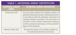
The individual dimensional elements of a microstrip antenna array may vary and may be spatially configured in a linear, planar, or volumetric arrangement. The radiation pattern of an array is determined by the dimensions, spatial distribution, and electrical excitation, i.e., amplitude and phase, of the individual elements. Given the number of variables, a general approach to the synthesis and design of antenna arrays is clearly required. To that end, antenna specialists have been successful in formulating a general methodology using the definitions in Table 1.
The product of the array factor and the element factor is referred to as the pattern multiplication theorem. An example will illustrate the convenience and efficiency of the theorem.
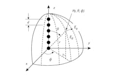
1. The linear array of isotropic radiating elements is depicted.
Consider the linear distribution of equally spaced, isotropic radiating elements along the z-axis (Fig. 1). The E-field radiation pattern of the ith element may be written as:1

The following definitions are applicable to this equation:
F(θ,ɸ) represents the radiation pattern of the element, and k0 = 2π/λ0, Ii, and βi are the amplitude and phase excitation.
For n identical elements, the radiation pattern is written as:

The radiation pattern is the product of the two terms:
F(θ,ɸ) is the element factor (EF), and

is the array factor (AF).
The perceptive reviewer may recognize the similarity between the array factor and the discrete Fourier transform of the complex linear distribution of amplitude and phase of the radiating elements. For the specified equally spaced condition and progressive phase of each element, one may write:

and

If the indicated substitutions are implemented, the array factor may be written:

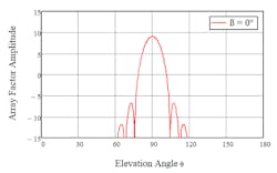
Solution of the equation using constant amplitude distribution (Ii = 1.0), parametric phase progression (β0 = 0, β0 = −π/4, β0 = π/4), number of elements (n = 16), and element spacing (d = λ0/2) is graphically illustrated within Figure 2.
The maximum amplitude of the array factor occurs at θ = 90 degrees for 0-degree phase excitation; at 105 degrees for 45-degree phase progression; and at 75 degrees for −45-degree phase progression. Clearly, the phase progression excitation enables the significant property of main beamsteering of antenna arrays. An additional observation is that the array of isotropic radiating elements has provided focus, i.e. gain, over the single element. In this instance, the numeric gain is equal to the number of array elements, n.
Another observation from Figure 2 is the sin(x)/x amplitude function. This behavior might have been anticipated due to the constant amplitude-element excitation and the discrete Fourier transform relationship.
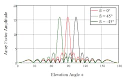
2. This figure illustrates array factor for a linear array of isotropic elements.
Constant, or uniform, amplitude distribution has been considered to this point of the exercise. However, in addition to phase progression excitation, amplitude variation of the array elements also offers some interesting properties. Consider the graphic of Figure 3, where the array factor for constant amplitude element excitation is indicated in the top plot, while raised cosine element amplitude excitation has been implemented in the bottom plot.
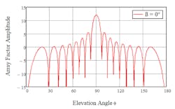
3. This array factor versus element amplitude variation (note logarithmic amplitude scale) comparison reveals constant amplitude excitation (top) and cosine amplitude excitation (bottom).
The raised cosine amplitude excitation of the array elements significantly reduced the array sidelobes. Unfortunately, the array amplitude also was reduced while the beamwidth increased. These are the significant tradeoffs when considering application of antenna-array implementation.
Microstrip antenna arrays will be further explored within the electromagnetic (EM) simulations in the upcoming sections. In many instances, the element spacing for most applications is approximately half-wavelength (λ0/2) in air. Although somewhat higher gain may be attained using element spacing beyond half-wavelength, increased sidelobe levels, particularly near ±90 degrees off-boresight (grating lobes), are a direct result. Therefore, in the simulations that will follow, element spacing in the plane of the antenna will be maintained at approximately half-wavelength.
Linear Microstrip Array Antennas
Figure 4 illustrates the configuration of a parallel-feed (alternately referred to as corporate feed) linear array composed of four in-line elements. Each element of the linear array is fed from the output of a power divider, which facilitates excitation of either equal or unequal power to each element. The power distribution to the elements of an array, as previously indicated, is commonly referred to as amplitude taper, and is utilized to reduce sidelobe levels. Amplitude taper is accompanied by increased beamwidth and reduced gain with respect to uniform, or equal, power distribution to each element.
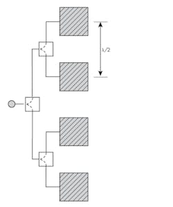
4. Here’s a four-element linear array.
The excitation to each element of the array may also be varied in phase. Progressive differential phase excitation is employed to steer the main beam off-boresight and is a unique and attractive feature for large phased-array radar applications as an alternative to inertial (mechanical) platforms.
A four-element linear array has been constructed using the single-element, 5.80-GHz microstrip antenna previously described and analyzed. The data from EM analysis of the four-element array is summarized in Table 2.

Table 3 documents the performance of a four-element linear array that has an amplitude taper applied to it. As mentioned previously, the amplitude taper is utilized to reduce sidelobe levels. The amplitude taper is implemented by changes to the impedance of the power divider’s lines in a manner that alters the impedance at the principal junction of the power divider. A simple equation governs the power-divider design under the specified conditions.3

Table 4 illustrates the configuration of a two-×-two array. The two-×-two array excitation is generally uniform; the most prominent feature is that the gain is typically 6 dB above the single-element configuration with the commensurate reduction in E-plane and H-plane beamwidth. In this case, the gain, 11.45 dB, is limited due to the inclusion of line and impedance-mismatch loss. The conductor current discloses that each element of the array is uniformly excited in amplitude and phase.
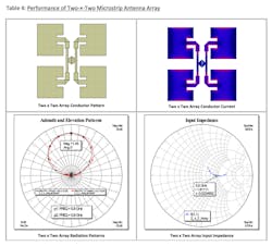
The differential feed at the center of the conductor pattern may be implemented from a balun located below the plane of the array. Differential feed is required in this case due to the inverse polarity of the radiating edges. The input impedance is 100 Ω at the center frequency, which is commensurate with typical balun impedance.
The individual excitation parameters of amplitude and phase determine the principal radiation intensity beamwidth, gain, direction, and sidelobe level. Clearly, antenna arrays are significant performance determinants to communication and radar systems.
References
1. Bahl, I. J. and Bhartia, P., Microstrip Antennas, Chapter 7, Artech House, Dedham, Mass., 1980.
2. The current density annotation feature available within the AXIEM EM analysis software provides significant, physically insightful information. The graphic indicates that the amplitude and phase of the individual element excitation are equal. This feature is uniquely valuable in evaluation of proper amplitude and phase excitation of more complex array structures.
3. The unequal power divider is documented at the website: http://www.microwaves101.com/encyclopedia/calpowerdivider.cfm.

