Algorithms to Antenna: Calibration Techniques for Phased-Array Antennas

When large phased-array antennas are built, perturbations in amplitude, phase, element position, and antenna patterns will invariably be present due to a range of factors. Perturbations can also arise due to other factors, such as coupling, hardware aging, clock drifting, and environmental effects. These perturbations may impact the performance of the system. In this blog, we review some simple examples that show how these imperfections can be modeled. We also look at some techniques that calibrate out these imperfections and improve system performance.
Note that while these examples are based on small linear arrays to help illustrate the ideas, the same type of workflows can be applied to larger, more complex array structures.
Modeling Array Perturbations
Figure 1 shows how perturbations in gain on a uniform linear array (ULA) affect the array pattern. Here, the perturbations are assumed to be statistically independent zero-mean Gaussian random variables with standard deviation of 0.1. Similarly, phase perturbations can be applied to the element tapers.
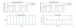
1. This figure depicts amplitude and phase perturbations in a uniform linear array.
Note how the pattern responses have shallower nulls for the perturbed arrays compared with the ideal system.
This same type of comparison can be made when the positions of the elements along all three axes are perturbed. Figure 2 shows the resulting pattern, which is impacted much more outside the main lobe.
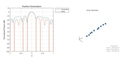
2. Shown are perturbed element positions across three axes.
An isotropic antenna element was used in the previous examples. We can replace this ideal antenna element pattern with a perturbed pattern. The results are shown in Figure 3.
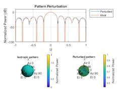
3. Perturbations in the antenna element pattern are illustrated.
Again, the main difference for this case is in the depth of the nulls that are generated.
Pilot Calibration
Once we have a model of a perturbed phased-array antenna, we’re able to perform calibrations to help account for (and correct) the imperfections. It’s critical to calibrate the array before its deployment. Calibration is also performed regularly in all deployed systems.
We will start with a technique referred to as pilot calibration. With pilot calibration, the focus is on estimating the location of the perturbations, based on the response of the array to one or more known external sources at known locations. You can compare the effect of perturbations on the array performance before and after the calibration.
Similar to what was described earlier, we start with an array that has amplitude, phase, and element position distortions (Fig. 4).
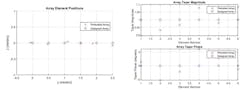
4. Phased array with amplitude, phase, and position perturbations is revealed here.
Now consider the case of a beamformer designed to steer the ideal array to a direction of 10 degrees azimuth with two interference sources from two known directions (−10 degrees azimuth and 60 degrees azimuth). The goal is to preserve the signal of interest while suppressing the interference sources.
Figure 5 compares the expected beam pattern with the pattern that results from applying the designed weights on both the ideal and the perturbed array.
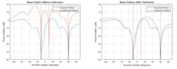
5. This is a comparison of non-calibrated and calibrated beam pattern.
The pattern generated using the uncalibrated weights does not satisfy the requirements because a null occurs around the desired 10 degrees azimuth direction. This means that the desired signal can no longer be retrieved. The plot on the right side of Figure 5 shows the calibrated response, which does preserve the desired signal.
Self-Calibration
It’s also possible to implement a self-calibration procedure based on a constrained optimization process. With this technique, opportunistic sources are used to simultaneously estimate array-shape perturbations and source directions. Self-calibration is more challenging to solve in general, as there are more unknowns.
With self-calibration (also called autocalibration), perturbations are estimated jointly with the positions of various external sources at unknown locations. Unlike pilot calibration, this approach results in a small number of signal observations with a large number of unknowns. One way to solve this problem is to construct and optimize against a cost function.
These cost functions tend to be highly nonlinear and contain local minima. In the example below, a cost function based on the Multiple Signal Classification (MUSIC) algorithm is formed and solved as an optimization problem. The cost function and optimization algorithm are chosen to achieve a solution as easily and quickly as possible. In addition, parameters associated with the optimization algorithm must be tuned for the given scenario. A number of cost function and optimization algorithms exist in the literature. For this scenario, a MUSIC cost function is chosen alongside an optimization algorithm.
As a scenario changes, you may need to adapt the approach used depending on the robustness of the calibration algorithm. For example, the calibration algorithm’s performance drops as sources move away from the array end-fire. It can also drop as the number of array elements increase.
Figure 6 shows the array that’s used in this example. Note in this figure, “Deployed Array” describes the ideal/intended element positions.
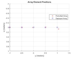
6. Shown are the different array element positions.
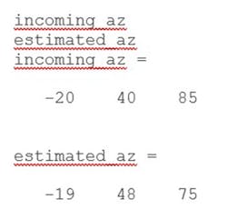
For this example, a beamscan estimator is used to estimate the directions of three unknown sources at −20, 40, and 85 degrees azimuth. The estimated azimuth angles are also shown.
These perturbations degrade the array’s performance. Self-calibration enables the array to be recalibrated using opportunistic sources without knowledge of their locations. Figure 7 shows results of how the calibrated array can be used to match the perturbed array.
7. These are calibrated array positions.
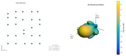
Figure 8 shows the results of the calibration process, revealing much improved accuracy of the source estimation. In addition, the positions of the perturbed sensors have also been estimated, which can be used as the new array geometry in the future.
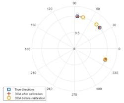
8. Direction of Arrival (DOA) angles before and after calibration are depicted.
Summary
A range of uncertainties and perturbations can impact the performance of an array. If you’re able to model these perturbations, you can also get a head start on developing calibration techniques before a system is fielded. Many additional technical references will help in this process.
To learn more about the topics covered in this blog, see the links below or email me at [email protected].
- Modeling Perturbations and Element Failures in a Sensor Array (example): Learn how to model amplitude, phase, position, and pattern perturbations, as well as element failures, in a sensor array.
- Using Self Calibration to Accommodate Array Uncertainties (example): Learn how to perform self-calibration based on a constrained optimization process.
- Using Pilot Calibration to Compensate for Array Uncertainties (example): Learn how to use pilot calibration to improve the performance of an antenna array in the presence of unknown perturbations.
See additional 5G, radar, and EW resources, including those referenced in previous blog posts.

About the Author
Rick Gentile
Product Manager, Phased Array System Toolbox and Signal Processing Toolbox
Rick Gentile is the product manager for Phased Array System Toolbox and Signal Processing Toolbox at MathWorks. Prior to joining MathWorks, Rick was a radar systems engineer at MITRE and MIT Lincoln Laboratory, where he worked on the development of several large radar systems. Rick also was a DSP applications engineer at Analog Devices, where he led embedded processor and system level architecture definitions for high performance signal processing systems used in a wide range of applications.
He received a BS in electrical and computer engineering from the University of Massachusetts, Amherst, and an MS in electrical and computer engineering from Northeastern University, where his focus areas of study included microwave engineering, communications, and signal processing.
Honglei Chen
Principal Engineer
Honglei Chen is a principal engineer at MathWorks where he leads the development of phased-array system simulation. He received his Bachelor of Science from Beijing Institute of Technology and his MS and PhD, both in electrical engineering, from the University of Massachusetts Dartmouth.
