Identify Modulation for Communications and Radar Using Deep Learning
Download this article in PDF format.
We also want to recognize Rick Gentile of MathWorks as a co-author of this article.
Modulation identification is an important function for an intelligent receiver. It has numerous applications in cognitive radar, software-defined radio, and efficient spectrum management. To identify both communications and radar waveforms, it’s necessary to classify them by modulation type. For this, meaningful features can be input to a classifier.
While effective, this procedure can require extensive effort and domain knowledge to yield an accurate classification. This article will explore a framework to automatically extract time-frequency features from signals. The features can be used to perform modulation classification with a deep-learning network. Alternate techniques to feed signals to a deep-learning network will be reviewed.
To support this workflow, we will also describe a process to generate and label synthetic, channel-impaired waveforms. These generated waveforms will in turn provide the training data that can be used with a range of deep-learning networks. Finally, we will describe how to validate the resulting system with over-the-air signals from software-defined radios (SDR) and radars.
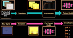
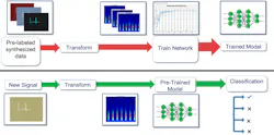
Figure 1 shows the workflow, which results in modulation identification and classification.
1. This modulation identification workflow with deep learning uses MATLAB. (© 1984–2019 The MathWorks, Inc.)
Challenges of Modulation Identification
Modulation identification is challenging because of the range of waveforms that exist in any given frequency band. In addition to the crowded spectrum, the environment tends to be harsh in terms of propagation conditions and non-cooperative interference sources. When doing modulation identification, many questions arise including:
- How will these signals present themselves to the receiver?
- How should unexpected signals, which haven’t been received before, be handled?
- How do the signals interact/interfere with each other?
Machine- and deep-learning techniques can be applied to help with modulation identification. To start, consider the tradeoff between the time required to manually extract features to train a machine-learning algorithm versus the large data sets required to train a deep-learning network.
Manually extracting features can take time and requires detailed knowledge of the signals. On the other hand, deep-learning networks require large amounts of data for training purposes to ensure the best results. One benefit of using a deep-learning network is that less pre-processing work and manual feature extraction is needed.
With the requirements for perception generally growing for autonomous driving and computer vision, great investments continue to be made on image- and vision-based learning. These investments can be leveraged by other signal-based applications such as radar and communications. This is true whether the data sets include raw data or pre-processed data.
In the examples described below, deep-learning networks perform the “heavy lifting” in terms of classification, so the focus is on the best way to satisfy the data set requirements for training and validation. Data can be generated from fielded systems, but it can be challenging to collect and label this data.
Keeping track of waveforms and syncing transmit and receive systems results in large data sets that can be difficult to manage. It’s also a challenge to coordinate data sources that aren’t geographically co-located, including tests that span a wide range of conditions. In addition, labeling this data either as it’s collected or after the fact requires much work, because ground truth may not always be available or reliable.
Another option is to use synthetic data, because it can be much easier to generate, manage, and label. The question is whether the fidelity of the synthetic data is sufficient. In the use cases that follow, we will show that generating high-fidelity synthetic data is possible.
Synthesizing Radar and Communications Waveforms
In our first example, we classify radar and communications waveform types based on synthetic data. As previously noted, the occupied frequency spectrum is crowded and transmitting sources such as communications systems, radio, and navigation systems all compete for spectrum. To create a test scenario, the following waveforms are used:
- Rectangular
- Linear frequency modulation (LFM)
- Barker code
- Gaussian frequency shift keying (GFSK)
- Continuous phase frequency shift keying (CPFSK)
- Broadcast frequency modulation (B-FM)
- Double sideband amplitude modulation (DSB-AM)
- Single sideband amplitude modulation (SSB-AM)
With these waveforms defined, functions are used to programmatically generate 3,000 IQ signals for each modulation type. Each signal has unique parameters and is augmented with various impairments to increase the fidelity of the model. For each waveform, the pulse width and repetition frequency are randomly generated. For LFM waveforms, the sweep bandwidth and direction are randomly generated.
For Barker waveforms, the chip width and number are randomly generated. All signals are impaired with white Gaussian noise. In addition, a frequency offset with a random carrier frequency is applied to each signal. Finally, each signal is passed through a channel model. In this example, a multipath Rician fading channel is implemented, but other models could be used.
The data is labeled as it’s generated in preparation to feed the training network.
Feature Extraction Using Time-Frequency Techniques
To improve the classification performance of learning algorithms, a common approach is to input extracted features in place of the original signal data. The features provide a representation of the input data that makes it easier for a classification algorithm to discriminate across the classes.
In practical applications, many signals are nonstationary. This means that their frequency-domain representation changes over time. One useful technique to extract features is the time-frequency transform, which results in an image that can be used as an input to the classification algorithm. The time-frequency transform helps to identify if a particular frequency component or intermittent interference is present in the signal of interest.
Many automated techniques are available for time-frequency transforms, including spectrogram and continuous wavelet transforms (CWT). However, we will use the Wigner-Ville distribution (WVD) because it provides good spectral resolution without leakage effects of other techniques.
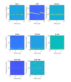
The Wigner-Ville distribution represents a time-frequency view of the original data that’s useful for time-varying signals. The high resolution and locality in both time and frequency provide good features for the identification of similar modulation types. We compute the smoothed pseudo WVD for each of the modulation types. This is because for signals with multiple frequency components, the WVD performance degrades due to cross terms. The down-sampled images are shown in Figure 2 for one set of data.
2. Time-frequency representations of radar and communications waveforms. (© 1984–2019 The MathWorks, Inc.)
These images are used to train a deep convolutional neural network (CNN). From the data set, the network is trained with 80% of the data and tested on 10%. The remaining 10% is used for validation.
Set Up and Train the Deep-Learning Network
Before the deep-learning network can be trained, the network architecture must be defined. The results for this example were obtained using transfer learning with AlexNet, which is a deep CNN created for image classification. Transfer learning is the process of retraining an existing neural network to classify new targets. This network accepts image inputs of size 227-by-227-by-3. AlexNet performs classification of 1,000 categories in its default configuration. To tune AlexNet for this data set, we modify the final three classification layers so that they classify only our eight modulation types. This workflow also can be accomplished with other networks such as SqueezeNet.
Once the CNN is created, training can begin. Due to the data set's large size, it may be best to accelerate the work with either a GPU or multicore processor. Figure 3 shows the training progress as a function of time using a GPU to accelerate the training. Training progress is expressed as accuracy as a function of the number of iterations. The validation accuracy is over 97% after epoch 5.
3. A GPU is used to accelerate the training process. (© 1984–2019 The MathWorks, Inc.)
Evaluating the Performance
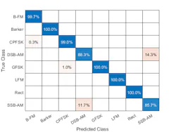
Recall that we saved 10% of the generated data for testing. For the eight modulation types input to the network, over 99% of B-FM, CPFSK, GFSK, Barker, Rectangular, and LFM modulation types were correctly classified. On average, over 85% of AM signals were correctly identified. From the confusion matrix, a high percentage of DSB-AM signals were misclassified as SSB-AM and SSB-AM as DSB-AM (Fig. 4).
4. The confusion matrix reveals the results of the classification. (© 1984–2019 The MathWorks, Inc.)
The framework for this workflow enables the investigation of the misclassifications to gain insight into the network's learning process. Since DSB-AM and SSB-AM signals have a very similar signature, this explains in part the network’s difficulty in correctly classifying these two types. Further signal processing such as the CWT could make the differences between these two modulation types clearer to the network and result in improved classification. Specifically, the CWT offers better multi‐resolution analysis, which provides the network with better information related to abrupt changes in the frequency of the signals.
This example showed how radar and communications modulation types can be classified by using time-frequency signal-processing techniques and a deep-learning network. In the second example, we will look at other techniques to input data into the network. Furthermore, we will use data from a radio for the test phase.
Alternate Approaches
For our second approach, we generate a different data set to work with. The data set includes the following 11 modulation types (eight digital and three analog):
- Binary phase-shift keying (BPSK)
- Quadrature phase-shift keying (QPSK)
- 8-ary phase-shift keying (8-PSK)
- 16-ary quadrature amplitude modulation (16-QAM)
- 64-ary quadrature amplitude modulation (64-QAM)
- 4-ary pulse amplitude modulation (PAM4)
- Gaussian frequency-shift keying (GFSK)
- Continuous phase frequency-shift keying (CPFSK)
- Broadcast FM (B-FM)
- Double-sideband amplitude modulation (DSB-AM)
- Single-sideband amplitude modulation (SSB-AM)
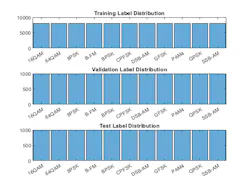
In this example, we generate 10,000 frames for each modulation type. Again, 80% of the data is used for training, 10% is used for validation, and 10% is used for testing as shown in Figure 5.
5. The distribution of labeled data is set by waveform type. (© 1984–2019 The MathWorks, Inc.)
For digital modulation types, eight samples are used to represent a symbol. The network makes each decision based on single frames rather than on multiple consecutive frames. Similar to our first example, each signal is passed through a channel with additive white Gaussian noise (AWGN), Rician multipath fading, and a random clock offset. We then generate channel-impaired frames for each modulation type and store the frames with their corresponding labels.
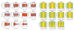
To make the scenario more realistic, a random number of samples are removed from the beginning of each frame to remove transients and to make sure that the frames have a random starting point with respect to the symbol boundaries. The time and time-frequency representations of each waveform type are shown in Figure 6.
6. Shown are examples of time representation of generated waveforms (left) and corresponding time-frequency representations (right). (© 1984–2019 The MathWorks, Inc.)
Train the CNN and Evaluate the Results
For this example, a CNN that consists of six convolution layers and one fully connected layer is used. Each convolution layer except the last is followed by a batch normalization layer, rectified-linear-unit (ReLU) activation layer, and max pooling layer. In the last convolution layer, the max pooling layer is replaced with an average pooling layer. To train the network, a GPU is used to accelerate the process.
In the previous example, we transformed each of the signals to an image. For this example, we look at an alternate approach where the I/Q baseband samples are used directly without further preprocessing.
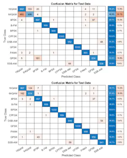
To do this, we can use the I/Q baseband samples in rows as part of a 2D array. In this case, the convolutional layers process in-phase and quadrature components independently. Only in the fully connected layer is information from the in-phase and quadrature components combined. This yields a 90% accuracy.
A variant on this approach is to use the I/Q samples as a 3D array where the in-phase and quadrature components are part of the third dimension (pages). This approach mixes the information in the I and Q evenly in the convolutional layers and makes better use of the phase information. The variant yields a result with more than 95% accuracy. Representing I/Q components as pages instead of rows can improve the network’s accuracy by about 5%.
As the confusion matrix in Figure 7 shows, representing I/Q components as pages instead of rows dramatically increases the ability of the network to accurately differentiate 16-QAM and 64-QAM frames and QPSK and 8-PSK frames.
7. Results with I/Q components are represented as rows (top) and as pages (bottom). (© 1984–2019 The MathWorks, Inc.)
Testing with SDR
In the first example we described (with radar and communications signals), we tested the trained network using only synthesized data. For the second example, we use over-the-air signals generated from two ADALM-PLUTO radios that are stationary and configured on a desktop (Fig. 8). The network achieves 99% overall accuracy. This is better than the results obtained for synthetic data because of the simple configuration. In addition, the workflow can be extended for radar and radio data collected in more realistic scenarios.
8. The SDR configuration uses ADALM-PLUTO radios (left). Also shown is the corresponding confusion matrix (right). (© 1984–2019 The MathWorks, Inc.)
Summary
Frameworks and tools exist to automatically extract time-frequency features from signals. These features can be used to perform modulation classification with a deep-learning network. Alternate techniques to feed signals to a deep-learning network are also possible.
It’s possible to generate and label synthetic, channel-impaired waveforms that can augment or replace live data for training purposes. These types of systems can be validated with over-the-air signals from software-defined radios and radars.
For more detailed description including MATLAB scripts on the above examples, see:
- Radar Waveform Classification Using Deep Learning (example)
- Modulation Classification with Deep Learning (example)
For questions on this topic, please email Rick Gentile at [email protected].
Ethem Sozer is Principal Software Engineer, Honglei Chen is Principal Software Engineer, Matt Sprague is Software Engineer, Sara James is Software Engineer, and Rick Gentile is Product Manager at MathWorks.
About the Author
Ethem Sozer
Principal Software Engineer
Honglei Chen
Principal Engineer
Honglei Chen is a principal engineer at MathWorks where he leads the development of phased-array system simulation. He received his Bachelor of Science from Beijing Institute of Technology and his MS and PhD, both in electrical engineering, from the University of Massachusetts Dartmouth.
