Estimating the Crest Factor (Peak-to-RMS Ratio) for a Sum of Sinusoidal Signals
What you'll learn:
- RMS, peak-to-peak, and peak-to-RMS of sinusoidal signals.
- Crest factor for a sum of sinusoids ≈ Gaussian distribution.
- What’s the central limit theorem?
- How the central limit theorem applies to continuous functions.
- Computing the peak-to-RMS ratio for a sum of up to N sinusoids with random parameters.
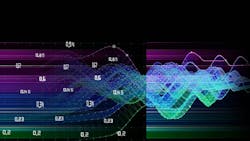
- Example of sinusoidal sums in temporal and frequency domains.
- Peak-to-RMS simulation results.
The crest factor, or peak-to-RMS ratio, is a signal metric to quantify the dynamic range of a signal. It provides a link between its RMS value and its peak value. Because the RMS value is often known or easily measurable, the crest factor provides a means of quickly estimating its peak value.
It’s often used when specifying an analog-to-digital converter (ADC) to avoid exceeding the range of the converter, yet still provides sufficient resolution of the signal about its RMS value. The parameter is also useful in data-recovery applications to estimate the peak-to-peak jitter from its RMS value to avert bit errors or when specifying an amplifier to avoid intermodulation distortion at signal peaks.
For a random signal with a Gaussian probability distribution, the peak-to-RMS ratio depends on the sample size and isn’t limited to a maximum value. For example, with a sample size of 1,000, the average peak-to-RMS value will be about 3.3. If the sample size increases to 10,000, the average peak-to-RMS value rises to about 3.9.
For a bounded deterministic signal, the peak-to-RMS value can usually be computed and has a maximum value. For the sum of bounded deterministic signals, the behavior of the peak-to-RMS ratio as a function of the number of addends isn’t as clear.
One case of interest is the sum of sinusoids of various amplitudes and frequencies. This type of signal is frequently observed in the phase-noise characteristic of a signal or the frequency spectrum of a mixer. In the case of phase noise, each tone contributes to the total deterministic jitter. Although the total RMS value of the tones can be computed, the peak-to-peak value can’t be determined from the phase-noise data.
However, if the peak-to-RMS ratio for a sum of random sinusoids is known, then the peak-to-peak deterministic jitter can be estimated from its RMS value. To this end, this article presents a study of the peak-to-RMS ratio for a sum of sinusoids with random parameters.
References 1 and 2 suggest the central limit theorem may be used to determine the nature of a sum of bounded deterministic functions. We include a discussion of the validity of using the central limit theorem in this application.
RMS, Peak-to-Peak, and Peak-to-RMS of Sinusoidal Signals
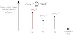
Equation 1 relates the RMS value of a single sinusoid to its amplitude Ao. For the sample of a signal composed of the sum of N sinusoids with different frequencies, and where multiple periods of each frequency are in the sample, Equation 2 relates its RMS value to the RMS value of each individual sinusoid.
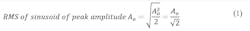

This relationship follows since the total power of a sum of sinusoids at different frequencies is the sum of the power of each of its component sinusoids as illustrated in Figure 1.
The peak-to-peak value of a single sinusoid is related to its RMS value by Equation 3 and its peak-to-RMS ratio is a constant as shown in Equation 4. However, the peak-to-peak value of a sum of N arbitrary amplitude, phase, and frequency sinusoids isn’t uniquely related to its RMS value. Intuitively, the phases and frequencies of the various sinusoids can add constructively or destructively and the amplitude of one or more tones may dominate. Hence, the peak-to-peak value isn’t simply the sum of the individual peak-to-peak sinusoids.


Crest Factor for a Sum of Sinusoids ≈ Gaussian Distribution
A review of the literature for the crest factor of a sum of sinusoids suggests that the sum should approach a Gaussian distribution. Specifically, Reference 1 includes the statement:
“According to the central limit theorem, the overall effect of a number of bounded sources would have a Gaussian distribution...”
Reference 2 adds:
“If a great number of small deterministic jitter1 (DJ) sources affect the signal, the overall effect of these bounded sources, according to the central limit theorem, will follow a Gaussian distribution that could be recognized as random jitter1 (RJ) contribution.”
However, the use of the central limit theorem to describe the nature of a set of continuous bounded sources isn’t a common use of the theorem as it typically applies to sets of discrete random variables. The following section reviews the central limit theorem and explores this possibility in greater detail.
What’s the Central Limit Theorem?
Each of these references cite the central limit theorem. It states that the distribution of a sum of independent random variables Xi, each with mean µi and variance σ2i under certain general conditions, approaches a Gaussian distribution with a mean of µ = µ1 + µ2 + … µN and variance σ2 = σ21 + σ22 + … σ2N (Reference 3).
As an example of the proper use of the central limit theorem, consider the values of N sinusoids at a common time instant. We’ll choose amplitudes, frequencies, initial phases, and start times of each sinusoid from uniform random distributions. Each individual sample at a single time instant is independent of any other samples at that same time instant, and the ensemble at that time instant are random. Therefore, the central limit theorem states that the distribution of these values at any time instant will approach a Gaussian distribution.
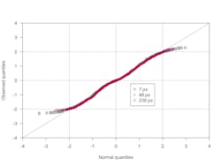
Figure 2 illustrates the histograms for the values of the sinusoids at times of 7 ps, 98 ps, and 238 ps. Although the sinusoid parameter values are based on uniform distributions, each distribution of 1,000 samples appears like a Gaussian distribution.
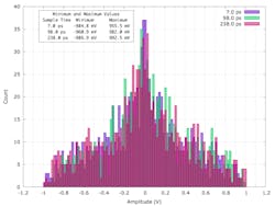
Figure 3 shows a more quantitative comparison of each distribution with its respective normal distribution of the same mean and standard deviation in a Q-Q plot. This plot indicates the three distributions are reasonably well approximated by Gaussian distributions and serve as valid examples of the central limit theorem.
However, the references state the central limit theorem may be used to determine the nature of a sum of N continuous functions and not a set of N independent random variables. The following section discusses whether this is a valid application of the central limit theorem.
How the Central Limit Theorem Applies to Continuous Functions
In the example of the sum of N sinusoids with uniformly distributed amplitudes, frequencies, initial phases, and start times, each sinusoid has a peak amplitude and RMS value. The peak-to-RMS value for the sum of 1,000 sinusoids is 4.66.
If one is using the central limit theorem to estimate the distribution of the sum of sinusoids, then the peak-to-RMS ratio of the sum should reflect the peak-to-RMS ratio for a Gaussian distribution. The mean value of the extreme value function for a set of 1,000 random Gaussian numbers is about 3.3σ and represents a mean peak-to-RMS ratio of 3.3. This isn’t consistent with the peak-to-RMS of the sum of 1,000 random sinusoids.
>>Download the PDF of this article
Consider the frequency-domain characteristic of the sum of 1,000 sinusoids as shown in Figure 4. The spectrum appears relatively flat over frequency. However, this doesn’t imply that the probability distribution must be Gaussian in nature. A flat frequency spectrum only indicates that the power is uniform over a range of frequencies.
To better understand the nature of the distribution of a sum of sinusoids relative to a Gaussian distribution, Figure 5 compares the peak-to-RMS ratios of sinusoidal sums of up to 1,000 sinusoids with that for a normal distribution of up to 1,000 samples. It also includes the mean expected value (50% probability) of the peak-to-RMS ratio for a normal distribution as a function of its sample size based on its extreme value function. The mean values are consistent with the results of the normally distributed values.
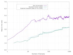
The peak-to-RMS ratio of a normal distribution has a positive slope over the entire range of 1,000 samples while the slope of the peak-to-RMS ratio for the sum of sinusoids saturates after about 100 sinusoids.
What’s evident from these observations is that the distribution of a sum of random sinusoids isn’t well modeled by a Gaussian distribution. Using the central limit theorem to estimate the properties of a large sum of sinusoidal signals doesn’t appear to be a proper interpretation of the theorem.
Therefore, we performed a set of simulations using sums of between 1 and 1,000,000 (16) sinusoids with random amplitudes, frequencies, initial phases, and start times, to study the nature of the distributions and establish a possible relationship between the sum of N sinusoids and their peak-to-RMS ratio. The following section includes a description of the study and summarizes its results.
Computing the Peak-to-RMS Ratio for a Sum of Up to N Sinusoids with Random Parameters
Studying the peak-to-RMS ratio of a sum of sinusoids requires an efficient means to compute a sum of between 1 and N sinusoids and to analyze each sum. This effort uses a compiled C program to compute the N f (t) sums, where each sum is of the form shown in Equation 5.

where:
- ti = start time in sec
- fi = frequency in Hz
- Ai = amplitude in V
- φi = initial phase in radians
For this set of analyses, we set the number of time samples of each sum to 220 and the time interval between samples to 1 ps for a total time span of 1.048576 µs. We advanced the number of sinusoids to sum, N, from 1 to 16. The sum of M sinusoids, where 2 ≤ M ≤ N, adds a sinusoid to the previous sum of M – 1 sinusoids to create the sum of M sinusoids. We also normalized the amplitude of each sum of M sinusoids to M and computed the peak-to-RMS value for each of the N sums.
Because the objective of this study is to determine the behavior of the peak-to-RMS ratio for a sum of sinusoids of arbitrary amplitudes, frequencies, initial phases, and start times, the simulation varied each of these parameters independently and randomly. We did, however, enforce limits on the range of some parameters because any real peak-to-RMS measurement has a finite measurement bandwidth, and its dynamic range is limited by measurement noise.
To avoid including a sinusoid whose period exceeds the total sample time of 1.048576 µs and avoid the effects of aliasing, we limited the range of frequencies to a minimum of 1/1.048576 µs ≈ 935.684 kHz and a maximum of 1/16 ps = 62.5 GHz (16 time samples per period). If the random frequency falls above the allowed maximum, the frequency is clamped to the maximum allowable frequency. If the frequency falls below the allowed minimum, an iterative process generates a new random frequency that falls above the minimum allowable frequency.
The dynamic range of the amplitudes is limited to about 35 dB by enforcing its value between 20 mV and 1.1 V. If the random amplitude exceeds 1.1 V, the amplitude is clamped to 1.1 V. If the amplitude is less than 20 mV, an iterative process generates a new random number that provides an amplitude greater than 20 mV.
The range of the initial phase is between 0 and approximately 2π radians, and the start times vary from about −500 ps to approximately +500 ps for a total range of about 1 ns. Varying the start time avoids phase coherence that occurs for small numbers of added sinusoids at the start of the simulation. Neither the initial phase nor the start time values are subjected to any limiting.
Each parameter is varied randomly using either a random uniform or a random Gaussian distribution. The sigma of the normalized Gaussian distribution is set to 1/6, and the range of the normalized uniform distribution is set to 1.0. The seed is based on the time stamp.
Example of Sinusoidal Sums in Temporal and Frequency Domains
Figure 6 illustrates two sums of 16 sinusoids in the time domain whose parameters are varied using uniform and Gaussian distributions. The statistical parameters for each waveform are included in the figure.
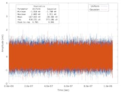
The RMS value of the sinusoidal sum whose parameters have a uniform distribution is slightly greater than the RMS value of the sum using parameters with a Gaussian distribution. This is expected because the probability of an amplitude close to the maximum amplitude of 1 V is greater with a uniform distribution than with a Gaussian distribution.
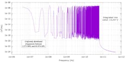
The power spectral density of the two sums is shown in Figure 7 with the integrated RMS value for each sum. The RMS values are consistent with those computed from the time-domain data in Figure 6.
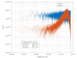
The flat frequency spectrum of the uniform distribution-based sum and the bell-shaped spectrum of the Gaussian distribution-based sum are consistent with the frequencies from a uniform and Gaussian frequency distribution.
Peak-to-RMS Simulation Results
We performed a total of 20 simulations for the sum of between 1 and 16 random sinusoids. Ten of the simulations used sinusoids with uniformly distributed parameters, and the remaining 10 used sinusoids with Gaussian distributed parameters. We then computed the peak-to-RMS values for each of the 20 simulations as a function of the number of sinusoids; they’re shown in Figures 10 and 11 of Reference 4.
We fit each of the 20 curves to an expression of the form of Equation 6. Coefficient co of Equation 6 represents the asymptotic value of f(x) when coefficient c2 is greater than 0.

- f(x) = peak-to-RMS ratio
- x = number of sinusoids
- ci = constants, I = 0, 1, 2
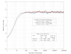
Figure 8 compares the average values for the two sets of simulations as a function of the number of sinusoids and their curve fit coefficients. The two average curves and their coefficients are essentially identical. The behavior of each as a function of the number of sinusoids is totally consistent with the result shown in Figure 5. As in that case, for large number of sinusoids, the peak-to-RMS ratio saturates to an asymptotic value of between 4.6 and 4.7.
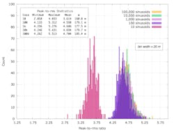
From Figures 12 and 13 of Reference 4, there’s some variation in the asymptotic value. To study the amount of variation in the peak-to-RMS value, we performed an analysis of the variation in the peak-to-RMS values for 1,000 sums of 10, 100, 1,000, 10,000, and 100,000 sinusoids using uniform distributed parameters.
The histogram in Figure 9 compares the distributions of the 1,000 peak-to-RMS values for each of the sums and includes a summary of their statistics. Sums of greater than 10 to 100 sinusoids have an average peak-to-RMS value of between 4.60 and 4.70 with an estimated standard deviation of about 0.180.
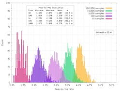
As further evidence that the use of the central limit theorem to estimate the nature of the sum of sinusoids distribution isn’t appropriate, Figure 10 shows the distributions of the peak-to-RMS values for 1,000 samples of 10, 100, 1,000, 10,000, and 100,000 Gaussian random numbers. As the number of samples increases, the average peak-to-RMS value doesn’t saturate but increases monotonically. This doesn’t provide an accurate model for the peak-to-RMS behavior for a sum of sinusoids.
The Bottom Line: Don’t Use the Central Limit Theorem to Estimate Peak-to-RMS Ratios
The equations for the RMS and peak-to-RMS values of a single sinusoidal signal are presented as the basis for illustrating that the peak-to-RMS value of the sum of an arbitrary number of random sinusoids isn’t easily computed. This article presented and reviewed earlier literature regarding the nature of the distribution for a sum of sinusoids in light of the central limit theorem.
We conducted a study of the peak-to-RMS ratio for sums of sinusoids with random amplitudes, frequencies, initial phases, and start times using both random uniform and random Gaussian distributions. A discussion covered the peak-to-RMS results as a function of the number of sinusoids in the sum for each distribution type. Those results are compared to the peak-to-RMS values for sets of Gaussian random numbers of the same size.
Unlike the Gaussian samples, the peak-to-RMS value for the sum of sinusoids is essentially bounded to its value at between 10 or 100 sinusoids. We’ve included equations and their coefficients relating the peak-to-RMS value to the number of sinusoids in the sum, based on curve fitting. The equations make it possible to quickly estimate the crest factor of a sum of N random sinusoids.
A more extensive description of the study with additional results is provided in Reference 4.
References
1. “The Uncertainty About Jitter,” Evaluation Engineering for Electronic Test and Measurement, August 1, 2012.
2. E. Balestrieri, L. De Vito, F. Lamonaca, F. Picariello, S. Rapuano and I. Tudosa, “The jitter measurement ways: The jitter decomposition,” in IEEE Instrumentation & Measurement Magazine, vol. 23, no. 7, pp. 3-12, Oct. 2020, doi: 10.1109/MIM.2020.9234759.
3. Papoulis, A. (1965) Probability Random Variables, and Stochastic Processes. McGraw-Hill Book Company, New York, London.
4. Logan, S. M, “Estimating the Crest Factor/Peak-to-RMS Ratio for a Sum of Sinusoidal Signals,” v1.2, October 25, 2024.
>> Download the PDF of this article
About the Author
Shawn Logan
Life Member, IEEE
Shawn M. Logan (Life Member, IEEE) started at Bell Laboratories in 1979. His fields of interest span frequency control devices, signal and system analysis, signal processing, analog circuit design, and simulation.
