One-Port VNA Calibration: A Look Under the Hood
Download this article in PDF format.
What you’ll learn:
- What is the three-term one-port VNA error model?
- Manipulation of an S-parameter flow diagram to allow for the determination of each network node in terms of a single dependent node.
- Solution of the three one-port error terms using a compact matrix solution of a system of three or more equations.
For a simple one-port vector-network-analyzer (VNA) calibration, only three error terms are needed: directivity (D), source match (S), and reflection tracking (R). These three errors theoretically appear between the VNA and the device under test (DUT). Knowledge of these three error terms allows for correction or calibration of the measurement.
Directivity error is mostly due to leakage in the bridge. Some amount of incident signal causes a small erroneous response on the reflection port. A typical raw bridge directivity might be anywhere from 15 to 40 dB. The source match represents the error in the source impedance of the VNA. The output source match is never perfect and is made somewhat worse by the cable connector and the test cable. A typical raw source match for a VNA might be 20 dB.
The reflection tracking error is basically the frequency response of the reflected signal from the DUT into the VNA and out through the reflection port of the bridge. This includes the loss incurred in the test cable and looks like a small value at low frequencies, increasing to several decibels at higher frequencies.
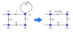
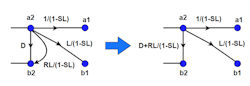
Figure 1 depicts a network-signal flow diagram with the three error terms included. A few simple manipulations of this diagram yield the formula for the measured value as a function of the DUT reflection coefficient and these three error terms.
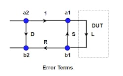
Note that b2/a2 is our measured reflection coefficient and b1/a1 is the actual reflection coefficient of L. We want to know b1/a1 while measuring b2/a2. This can be simplified with network flow-graph manipulations. For those unfamiliar with the technique, it involves only a few simple rules and an understanding that the math works only in the direction of a flow-graph arrow. For instance, from Figure 1, one can say that b2 = R * b1. It is NOT true that b1 = b2/R.
Network Flow-Graph Rules
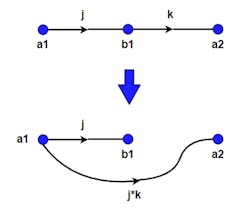
The first rule is the “Series Rule.” Because b1 = j * a1 and a2 = b1 * k, then a2 = j * k * a1 and one can break out the connection from a1 to a2 (Fig. 2). This is useful if a1 is the independent node in the network, as it now gives the other two nodes explicitly.
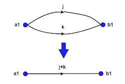
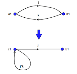
The next rule is the “Parallel Rule”: Because both branches “j” and “k” point in the same direction, their contributions may be combined as shown in Figure 3.
The next rule is the “Self-Loop Rule”: The loop is created by virtue of the Series Rule as the path from a1 to b1 and back may be combined (Fig. 4). This may not seem like a useful transform, but one more manipulation is possible. A network flow will always enter the loop. The loop may be removed, and its effect applied to that entering path as follows (Fig. 5).
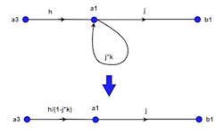
This transform comes from the parallel rule:

which reduces to:
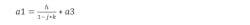
If the arrow from b1 pointed to the left and entered the loop, then “j” would have to be replaced by:

These rules may now be employed to simplify Figure 1 such that all nodes are explicitly defined by the single independent node “a2.” The steps encompass the transformation depicted in Figure 6, followed by the application of series and parallel rules as shown in Figure 7.
Finally, we see that our measured reflection coefficient is represented by:

We can solve this for L and obtain:
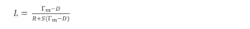
which is the result we were looking for.
Now, if we know D, R, and S, we can easily correct our Γm to obtain L, which is the actual reflection coefficient.
One-Port Calibration
We now make three measurements of three known artifacts and solve a system of equations to obtain the D, R, and S error terms. In addition, we could make more than three measurements and perhaps improve our estimation of the error terms with a least-squares approach. Rather than write out those three equations, we’ll jump right to the matrix notation, which is much cleaner.
Form two matrices, C and V:
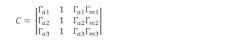
and
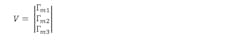
where the Γa values are the actual values and the Γm values are the measured values. We must know these actual values a priori. These could be an open, short. and load, where the actual values are characterized by short delays and parasitic capacitance or inductance as is done in a calibration kit. The three actual values could also be three shorts with different delays such that the three reflection coefficients are spread around the outside of the Smith chart over frequency.
Any three artifacts with known reflection coefficients may be used if they’re sufficiently separated on the Smith chart at every frequency. If they’re not, the matrix calculations will be ill-conditioned and the results unreliable.
With these two matrices, calculate matrix E:
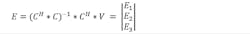
where H is the Hermetian transpose operator, or the matrix transposed with its entries conjugated.
From E, we can find D, R, and S: D = E2, S = E3, and R = E1 + E2 * E3
It so happens that (CH * C)−1 * CH is a least-squares calculation. If our measurements are a little noisy, we can improve our results by making more known measurements. Simply add more rows to the C and V matrices. Matrix E will still have three values in the end and the results might be somewhat better in the face of slightly noisy measurements.
Conclusion
In this article, we introduced the three-term error-correction terms, and used a simple method of derivation to show how these error terms affect the measured value. Finally, we outlined a simple matrix method for easy calculation of one-port error correction to arrive at calibrated results from the error terms. None of this work is original, but it’s educational to pull all of the pieces together and demonstrate how they are used.
References
Douglas Rytting, “Network Analyzer Error Models and Calibration Methods,” 62nd ARFTG Conference Short Course Notes, December 2-5, 2003, Boulder, Colo.
Feim Ridvan Rasim, Sebastion M. Sattler, “Analysis of Electronic Circuits with the Signal Flow Graph Method,” Scientific Research Publishing, Circuits and Systems, 2017, 8, 261-274
Jim Stiles, University of Kansas, Dept. of EECS, “4.5 – Signal Flow Graphs,” 3/19/2019, http://www.ittc.ku.edu/~jstiles/723/handouts/section_4_5_Signal_Flow_Graphs_package.pdf
About the Author
Brian Walker
Senior RF Engineer SME, Copper Mountain Technologies
Brian Walker is the Senior RF Engineer SME at Copper Mountain Technologies where he helps customers to resolve technical issues and works to develop new solutions for applications of VNAs in test and measurement.
Previously, he was the Manager of RF design at Bird Electronics, where he managed a team of RF Designers and designed new and innovative products. Prior to that he worked for Motorola Component Products Group and was responsible for the design of ceramic comb-line filters for communications devices. Brian graduated from the University of New Mexico, has 40 years of RF Design experience, and has authored three U.S. patents.
