Algorithms to Antenna: Reducing Signal Distortions—PA Characterization with DPD
I am excited this month to share a new workflow that I think will be useful in your wireless system design. The workflow provides a methodology you can use to characterize a nonlinear power amplifier (PA). It also connects this characterization to an adaptive digital pre-distortion (DPD) feedback system with an overall goal of reducing the effects of output signal distortion of an RF transmitter.
I like this workflow because you can use MATLAB to create a model for an RF PA. The coefficients of the model are extracted by fitting the actual measured data for the PA. After deriving the set of coefficients for the PA model with functions that operate on the measured data, you can use the model as part of a system-level simulation to see how performance changes with DPD.
To accomplish this, we provide an adaptive DPD algorithm that can be enabled during simulation. It’s able to help you evaluate and understand how the linearity of the RF transmitter system output signal improves after enabling DPD correction.
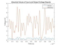
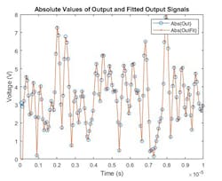
1. This figure illustrates the PA characterization.
Figure 1 shows the input and output complex measured I/Q signals of the PA that we started with. This commercially available PA was characterized in the lab using a standard-compliant LTE signal.
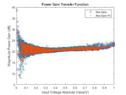
The top plot of Figure 2 shows the magnitude characteristic of the PA—the absolute value of the output gain versus input signals. Note that scattering around a straight line representing the gain results from memory effects (curve dispersion). The bending of the data curve for large input-signal values results from the PA nonlinearity (deviation from straight horizontal line).
2. Shown is the magnitude characteristic of the PA (top) and power gain transfer function of the PA (bottom).
With this data, we have multiple ways to determine the complex coefficients for the amplifier model. The bottom plot of Fig. 2 shows the resulting power gain transfer function for one technique using a generalized memory polynomial approach.
Once we have our coefficients, we can load them directly into our PA model, shown in Figure 3 as part of a system-level simulation.
3. This figure depicts a system-level model for 16-QAM waveform.
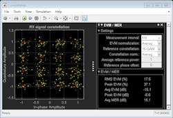
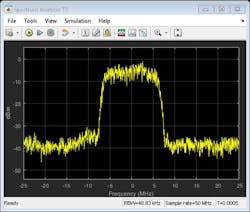
In Figure 4 (top), we can see that with DPD disabled, the average modulation error rate (MER) is about 15 dB.
4. A receive constellation for 16-QAM system is shown.
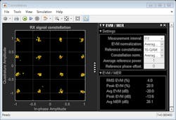
With DPD enabled, the average MER improves to 28 dB (Fig. 5).
5. Here’s a receive constellation for 16-QAM system with DPD enabled.
You can also implement the DPD algorithm on an FPGA or a microcontroller for rapid prototyping. With this approach, you can use the same testbench to test and implement your algorithm. I will talk more about this in a future blog.
Everything I have described quickly here is explained in more detail in the Power Amplifier Characterization with DPD for Reduced Signal Distortion example. In the full example, you can see a range of techniques to generate the coefficients. You can also see more info on the system-level model to see how DPD can be used to reduce the effect of the PA’s nonlinearities.
Have more questions? Email me at [email protected]
Learn more about the topics covered in this blog post:
- Power Amplifier Characterization with DPD for Reduced Signal Distortion (Example): Explore a methodology for characterizing a nonlinear RF Blockset PA with memory and an adaptive DPD feedback system to reduce the output signal distortion of an RF transmitter.
- Power Amplifier Modeling and DPD Design with MATLAB (Video): Learn how to develop different PA models, simulate the PA model in a closed-loop simulation, and develop DPD algorithms to improve the performance of an RF system.
- Modeling RF Power Amplifiers and Increasing Wireless Transmitter Linearity with DPD Using MATLAB (Webinar): Learn how to model RF PAs using measurement data, including nonlinear and memory effects. We will explore tradeoffs and white-box fitting techniques to increase PA model performance.
See additional 5G, radar, and EW resources, including those referenced in previous blog posts.
About the Author
Rick Gentile
Product Manager, Phased Array System Toolbox and Signal Processing Toolbox
Rick Gentile is the product manager for Phased Array System Toolbox and Signal Processing Toolbox at MathWorks. Prior to joining MathWorks, Rick was a radar systems engineer at MITRE and MIT Lincoln Laboratory, where he worked on the development of several large radar systems. Rick also was a DSP applications engineer at Analog Devices, where he led embedded processor and system level architecture definitions for high performance signal processing systems used in a wide range of applications.
He received a BS in electrical and computer engineering from the University of Massachusetts, Amherst, and an MS in electrical and computer engineering from Northeastern University, where his focus areas of study included microwave engineering, communications, and signal processing.

