This file type includes high resolution graphics and schematics when applicable.
Averaging is a common technique for reducing the measurement uncertainty inherent in all measurements. Performing the same measurement a number of times and averaging the results can reduce the randomness of the experimental result. Averaging is an automatic function available in most instruments. Rather than returning noise-ridden results, an instrument may make 100 measurements, calculate the average, and return just that average as the measured result. But power averaging in spectrum analyzers may actually provide misleading data as the following experiments intend to show.
The experiments involved correlating the power measurements of two spectrum analyzers from different vendors. However, the issues discussed are generic in the sense that they apply to any spectrum-analyzer power measurement with some form of post-detection averaging.
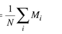
One of the first incorrect assumptions regarding power averaging in spectrum analyzers is averaging the root-mean-square (RMS) power will yield the average power of a zerospan trace or portion of the trace. Perhaps to understand the problem with this assumption, it may help to view averaging mathematically, as in Eq. 1. It shows MAVE as the average of a series of individual measurements taken over N trials of an experiment, where each of those measurements is denoted as Mi:
In this instance, the task was to verify that one instrument (instrument A) correlated with a second instrument (instrument B) to within some level of accuracy (for example 1 dB). All measurements were performed in zerospan (ZS) mode, a common spectrum-analyzer approach for measuring power at a specific frequency. The use of ZS is irrelevant to the problems with averaging, because the same kinds of averaging issues occur in traditional frequency-domain spectrum analysis.
In both cases, the ZS technique was used for adjacent-channel-power-ratio (ACPR) measurements. This measurement capability is common to modern analyzers with digital intermediate-frequency (IF) filters, allowing the instrument to perform multiple power measurements at varying offsets from the center frequency without retuning.
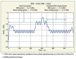
Figure 1 shows a real ZS measurement of a pulsed GSM signal. The blue curve represents the actual GSM pulse envelope. The measurement performed here is the "Output RF Spectrum (ORFS) due to modulation," which is simply an ACPR measurement.
It is possible to calculate a number of useful results from the trace, such as the maximum peak power, minimum power, and average power. Finding the trace maximum power and minimum power is conceptually straightforward the analyzer performs a maximum peak and minimum peak search on the entire trace and returns the results.
The simplest (and correct) way to calculate average power is to average across all the points between the red lines. Equation 2 accomplishes this, where N is the number of trace points between the red lines, and Pith point is power in the
Unfortunately, instrument manufacturers don't always agree on power averaging approaches. One of the instruments averaged powers as in Eq. 2, while the other instrument first converted each power point to a voltage, took the average of all of these voltages, and then used the average voltage to calculate the average power. Equation 3 shows this calculation:
It was not a trivial exercise to prove that one instrument was using Eq. 2 and the other was using Eq. 3 since the difference between the two reported average power levels wasn't that large. It was necessary to pull multiple traces out of both instruments and calculate the average every conceivable way until good fits were found. In the example in Fig. 1, the difference between the "true" average power (subsequently referred to as the RMS power) and the average voltage power is 0.25 dB (RMS power is 0.25 dB greater). This could have been written off as a simple measurement difference (error) between the two instruments. While 0.25 dB may not seem like much, when the requirement is for 1 dB of correlation (accuracy), 0.25 dB looms as a significant amount. If the difference in power levels over the whole burst is examined, the delta widens to ~1 dB (again, RMS power registering higher than average voltage power). In this case, the difference is equal to the level of accuracy one is trying to obtain.
Page Title
The average voltage power represents the "mean-squared" power (Eq. 3), while the RMS power is, obviously, the "mean-square" power (Eq. 2). From elementary statistics, it can be shown that the mean-square value minus the mean-squared value is equal to the variance. What this implies is that the amplitude variation (amplitude variance) will directly contribute to the difference in reported powers. Finally, the mean-square power will always be greater than or equal to the mean-squared power (RMS power > average voltage power).
A second incorrect assumption regarding power averaging is that average power is always calculated in linear terms, by averaging power in watts. In some cases, logarithmic averaging may be used, however. Continuing with the example, assume that many of the measurements suffer from noise. To remove some of the measurement noise, one may decide to apply an additional average: take multiple traces, compute each trace's average power, then average the powers across all traces (average of the averages). In the case of the GSM ORFS Mod measurement, the standard dictates that the power results are to be averaged over 200 bursts. Equation 4 shows the required calculation. To reiterate, each individual trace power (PTrace i) is a single number calculated with Eq. 2 or 3 (either RMS power or average voltage power):
It is reasonable to assume that the average will be computed with the PTrace i values in watts (referred to as linear averaging). However, many analyzers offer the ability to average logarithmically. In this case, power values in units of dBm are averaged. If, for example, given trace power averages of +1 and +3 dBm, the linear average would be (1.25 mW + 2 mW)/2 = 1.62 mW = +2.11 dBm. But the log average would be (1 dBm + 3 dBm)/2 = 2 dBm. Log averaging the numbers introduces an error of 0.11dB.
It should be noted that the size of the error introduced by logarithmic averaging depends upon whether the signal being measured is repetitive or not. In addition to the fact that averaging dBm values isn't really correct, there is a more subtle issuefor repetitive signals, linear and log averaging will produce the same result. Thus, logarithmic averaging a repetitive signal introduces no error. Note that a repetitive signal is defined as a signal that has the same power-versus-time trace for every sweep.
The fact that non-repetitive signals could produce different results is worth remembering, particularly because realworld operation conditions can differ from laboratory test conditions. Laboratory test signals are typically repetitive, given that they are often generated from a well-behaved arbitrary waveform generator (ARB) or similar digital signal generator. The ARB playsback the same waveform over and over again, so it's repetitive by definition. Real-world-signals are not, because they typically contain useful information that is changing in real time. However, provided there isn't a large difference in the average power from trace to trace, the differences between log and linear averaging are small.
Another observation worth noting it the use of point-to-point averaging to perform trace averaging on power measurements. In this case, the error introduced by logarithmic averaging also depends on the repetitiveness of the signal under test. In point-to-point averaging, multiple traces are collected, and each trace point is averaged against the corresponding points in all other traces.
Again, each point is averaged with all of the points that occur at the same x value, resulting in an "average" trace. For this discussion, x will be time, but it could be frequency, and the same results will apply. As before, the points can be averaged either linearly or logarithmically. Once the averaging is complete, an additional average can be applied to the whole trace or part of it. If the waveform is repetitive, linear and logarithmic averaging will give the same average trace, because for each and every trace a given point will have the same power.
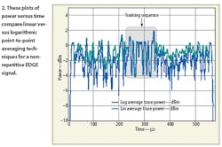
What happens when a waveform under test is not repetitive? Figure 2 shows the average traces for both linear and logarithmic power averaging taken over 20 bursts of an EDGE signal with varying payload data.
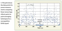
There is certainly a difference between the two traces, and it's obvious that the log-averaged trace has less power than the linear averaged trace. Figure 3 shows the difference between the two traces at every point.
Note that, as expected, the Training Sequence portion of the burst shows no difference between linear and log averaging.
The difference arises from the way that logarithmic averaging exaggerates power swings. This is best illustrated by a simple example. Assume one is measuring power at a specific point in time (or a specific frequency) over N bursts. The power is oscillating between two levels, for example, 0 dBm and 10 dBm; 50 percent of the power readings give 0 dBm, and 50 percent give 10 dBm. So, the peak-to-peak swing is 10 dB. What is the average power across the N bursts? Calculating the log answer is trivial: 5 dBm. To calculate the linear average, one converts 0 dBm and 10 dBm to values in watts, finds the average, and then converts this number back into dBm units. The average power in watts is 0.55 mW, or 2.6 dBm. Using log averaging introduces an error of 2.4 dB.
To generalize the calculation, it's known that an x dB change is equal to a change of 10(x/10) in linear power. Therefore, it is possible to write the following equation, again assuming that 50 percent of the points are at one level Mhi, and the other are Δ dB down from that level:
Page Title
Note that, as Δ goes to infinity, the term 10logΔ/10)/2> goes to 3 dB. This means that, in the case of equal numbers of two different power levels, the resulting average linear power will be at most 3 dB less than the higher power. It is possible to further generalize the result for an arbitrary ratio:
In Eq. 6, r is the ratio of the number of occurrences of the higher power (Mhi) to the total number of measurements. Note that when Δ goes to infinity, the resulting average power will be at most 10log(r) less than the higher power.
It is also possible to write the equation for the log average as:
If Eq. 7 is subtracted from Eq. 6, the result is an expression for the difference between linear averaging and log averaging (this is the error introduced by log averaging):
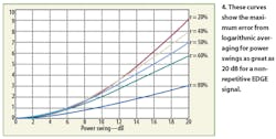
Figure 4 plots Eq. 8 vs. Δ for various values of r (Eq. 8). The plot was limited t o a Δ of 20 dB because this is likely to be at the upper end of common peak-to-average power ratio or crest factor values.
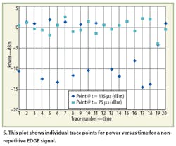
As a check, it might be helpful to look at a few points in some real data (refer back to Fig. 3). Here, two points in time are highlighted, one with a relatively large power difference (more than 3.5 dB at T = 115 s) and the other with a much smaller difference (~0.25 dB at T = 75 s). From the previous discussion, it would be reasonable to expect the corresponding power-versus-time plot for those points to look considerably different; the point with the high error should show quite a bit of power swing, while the low error point should show a smaller power swing. This is, in fact, the case, as seen in Fig. 5.
In Fig. 5, the trace corresponding to the point at T = 115 s has ~15 dB max amplitude swing, while the trace for the point at T = 75 s has ~5 dB of swing. If one assumes that the high and low values occur equally (i.e., r = 0.5), then the trace for T = 115 s should have a maximum error of ~4.5 dB, and the trace for T = 75 s should have a maximum error of ~0.5 dB (see Fig. 4 and Eq. 8). These values are greater than the measured 3.5 dB and 0.25 dB, but it's important to recall that the plot in Fig. 4 shows worst-case numbers (it assumes just two power levels, with equal numbers of each). One would expect the error to be smaller, since it's obvious that there are more than two values.
In summary, engineers should keep in mind that spectrum analyzers don't always adhere to the "correct" way of calculating average power. Furthermore, the size of the potential errors introduced depends on the characteristics of the signal being analyzed. In particular, it is important to:
- Understand the way the spectrum analyzer is calculating average power: RMS, voltage average, etc.
- Be aware that power isn't always averaged in linear units (watts), but that log averaging could be taking place.
- Repetitive signals can be misleading. The result may be either a static error (error is always the same and constant, for example, RMS versus average voltage) or no error (linear versus log averaging).
Differences in averaging techniques can lead to errors of 1.0 dB or more. The best way to understand how a particular spectrum analyzer calculates power averages is to pull a few traces out of the box and determine if manual calculations produce the same results as those produced by the analyzer. While this can be tedious, it is well worth the effort if an application requires high power measurement accuracy.
This file type includes high resolution graphics and schematics when applicable.
