The Differences Between Receiver Types, Part 1
This file type includes high resolution graphics and schematics when applicable.
Receivers undoubtedly play a critical role in any communications system. They perform the tasks of receiving an incoming transmitted signal and then recovering the information contained in those signals. Given the massive amount of information that is wirelessly communicated today, it is worthwhile to have a clear understanding of this subject.
This article, Part 1 of the series, provides a general overview of receivers. The direct-conversion receiver and the widely used superheterodyne receiver are both discussed here. Part 2, which will appear in the April issue of Microwaves & RF, will discuss the advantages and disadvantages of both implementations. In addition, the newer direct RF-sampling technique will be discussed in that second installment.
The Role of a Receiver
The input signal to a receiver is obtained from a receiving antenna. These received signals, which are typically very weak, can be described as modulated RF carrier signals. The modulation carries the actual information, which can be audio, video, or data. A receiver must perform a number of actions on a received signal so that the modulation information can ultimately be deciphered and processed.
Receivers are required to perform effectively despite the presence of noise and other interfering signals. Therefore, selectivity and sensitivity are important characteristics of one. Selectivity describes the capability of a receiver to identify and select a desired signal despite the presence of other unwanted signals. A receiver with good selectivity will process desired signals while sufficiently rejecting unwanted spurious and interference signals.
Sensitivity describes how well a receiver can process very weak input signals. It can be quantified as the weakest signal level that a receiver can detect to meet a given requirement, such as a specified signal-to-noise and distortion (SINAD) ratio or bit-error-rate (BER).
Sensitivity and Noise
Thermal noise represents the fundamental limit on achievable signal sensitivity. It is a result of the vibrations of conduction electrons and holes due to their finite temperature. The power delivered by a thermal source into a load is defined as:

where:
k = Boltzmann’s constant (1.38 x 10⁻²³ Joules/K);
T = temperature in degrees Kelvin (K);
B = noise bandwidth.
The standard source noise temperature, or To, is 290° K. Thus, the thermal noise generated in a 1-Hz bandwidth is:
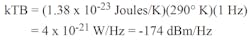
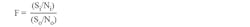
The noise floor sets the limit on the minimum detectable signal level. A noiseless receiver would therefore have a noise floor of -174 dBm/Hz. However, every receiver adds some amount of noise, further limiting its sensitivity. A receiver can be characterized by its noise factor (F), which is a measure of the degradation in the signal-to-noise ratio (SNR) as a signal passes through a network. It can be defined by the following equation:
where:
Si = the input signal power;
Ni = the input noise power;
So = the output signal power;
No = the output noise power.
Noise factor is therefore dependent on the source noise temperature as follows:

where:
To = standard noise source temperature (290° K);
NR = noise added by the receiver;
G = gain of the receiver.
The noise figure (NF) is simply the noise factor expressed in decibels:

The noise figure of a receiver can be determined by the gain and noise figure of its individual components. It can be calculated by the well-known equation for cascaded noise figure:
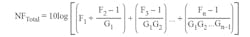
where:
F1 = noise factor of stage 1;
F2 = noise factor of stage 2;
Fn = noise factor of the nth stage;
G1 = gain of stage 1;
G2 = gain of stage 2;
Gn-1 = gain of stage n-1.
Direct-Conversion Receiver
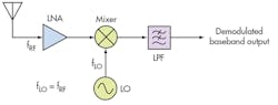
A direct-conversion receiver, also known as a homodyne or zero-IF receiver, is one type of receiver architecture (Fig. 1). Direct-conversion receivers convert an RF signal to a 0-Hz signal in one stage. They are generally considered low-cost solutions, as they require few components. In addition, they lend themselves well to integrated-circuit (IC) designs.
Direct-conversion receivers typically filter and amplify a received RF input signal. The signal then enters a mixer along with a local-oscillator (LO) signal that is identical in frequency to the RF input signal. Thus, the input signal is converted to a 0-Hz signal that appears at the output of the mixer. Demodulation occurs during the frequency conversion process, as well. Although the sum of the RF and LO signal frequencies also appears at the mixer’s output, this product is removed by means of low-pass filtering that follows the mixer. The demodulated baseband output is, of course, then processed.
Often, direct-conversion receivers are implemented with two mixers to create an in-phase/quadrature (I/Q) demodulator. The same LO drives both mixers. However, the LO signals to each mixer differ in phase by 90 deg. The I/Q signals can then be processed following the demodulation stage.
The Superheterodyne Receiver
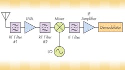
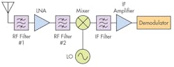
The superheterodyne receiver is a common receiver configuration that has been used for many years (Fig. 2). Superheterodyne receivers basically translate an RF input signal to a lower-frequency intermediate-frequency (IF) signal. The IF signal is then demodulated to allow the modulation data to be processed.
The entire process can be explained by analyzing the basic receiver shown in Fig. 2. (It should be noted that this receiver is only an example, as many variations can also be implemented.) A received signal first enters a bandpass filter. This filter, often called a pre-select filter, serves the purpose of rejecting out-of-band signals. Next, a low-noise amplifier (LNA) performs the task of boosting the signal amplitude. This LNA is an extremely important component, as the overall noise figure of a superheterodyne receiver is highly dependent on the noise figure of the LNA. Another bandpass filter, known as an image-reject filter, follows the LNA. The purpose of this filter is to reject the unwanted image frequency band.
A mixer then converts the RF signal to a lower-frequency IF signal. Both the RF signal and an LO signal enter the mixer, thereby generating the IF signal that appears at the mixer’s output. The frequency of this IF signal is equal to the difference of the RF input signal’s frequency and the LO signal’s frequency.
Following frequency downconversion, bandpass filtering is implemented in the IF stage to remove any unwanted signals. Next, an IF amplifier provides a significant amount of gain to the IF signal. Multiple amplifiers may be employed, as well. The amplified IF signal is then demodulated, allowing the information to be processed.
Superheterodyne receivers are often implemented with two frequency conversion stages. This configuration is particularly beneficial for higher-frequency applications. Part 2 of this series will pick up where this article leaves off by further examining dual-conversion superheterodyne receivers. The pros and cons of direct-conversion and superheterodyne receivers will be explained; some of the more recent receiver products will be mentioned, as well. Furthermore, the newer direct-RF sampling technique—an arena that holds great promise for future wireless systems—will be presented.
This file type includes high resolution graphics and schematics when applicable.
