Stripline Combline Filter Tunes 900 to 1,300 MHz

This file type includes high resolution graphics and schematics when applicable.
Filter designs are gaining in importance along with the growing number of wireless applications and occupied bandwidths. Bandpass filters with low passband loss and high rejection are needed throughout the wide expanse of wireless communications bands. This prompted an attempt to design a five-pole Chebyshev stripline combline bandpass filter (BPF) with a tunable center frequency. The tuning capability adds to the flexibility of the filter for different applications, while the stripline circuit technology supports high performance levels.
To demonstrate the feasibility of a stripline Chebyshev combline BPF, a circuit was fabricated on RO4003C substrate material from Rogers Corp. with dielectric constant of 3.38, using varactor diodes to achieve frequency tuning. The experimental filter covers a frequency range of 900 to 1,300 MHz while maintaining nearly constant fractional bandwidth.
Many RF/microwave filters are designed for use for different bands from 0.1 to 20.0 GHz.1 Tunable BPFs are of great interest for modern multiband communications systems, with many efforts made to decrease the size of these components.2 Such BPFs have been realized with a number of different topologies—including combline filters, which are compact and offer ease of integration with other circuits due to their planar implementation.3,4 A typical combline structure includes a series of transverse-electromagnetic (TEM) resonators with circular or rectangular cross-section and a capacitor for resonance at the open-circuit end of the structure.
The bandwidth and response of a combline filter is governed by the coupling of each resonator to its immediate neighbor. This is also a function of the resonator size, resonator spacing, and ground-plane separation.1 Different components and circuit elements are added to a combline BPF structure to tune the passband frequency, including PIN diodes,5 ferroelectric diodes,6 RF microelectromechanical systems (RF MEMS) devices,7 barium strontium titanate (BST) varactor diodes,8 and silicon/GaAs varactor diodes.9-13
Microstrip has been the basis for many tunable combline filter designs.14-21 In ref. 14, a tunable planar microstrip combline filter with multiresonator coupling is realized to achieve high selectivity. In ref. 15, a combline bandpass filter using step-impedance microstrip lines is investigated. Reference 16 details a 1.4-to-2.0 GHz miniature filter with high linearity. Reference 17 offers results on a tunable RF-MEMS microstrip filter with constant bandwidth by means of corrugated coupled resonators, while ref. 18 features a tunable combline bandpass filter loaded with series resonator.
Reference 19 details a compact dual-mode second-order filter with constant bandwidth, while ref. 20 presents a high-quality-factor (high-Q) fully reconfigurable tunable microstrip bandpass filter. Reference 21 details a tunable microstrip filter design with independent frequency and bandwidth control. All of these examples were based on microstrip. Few researchers have investigated stripline combline filters, although such filters can achieve much better bandwidth than their microstrip counterparts, with excellent isolation between adjacent traces.
To explore the performance capabilities of stripline combline filters, a five-pole stripline Chebyshev combline filter with tunable center frequency was designed and simulated. Tuning is performed by means of varactor diodes and capacitance that varies as a function of applied voltage. The filter provides tuning capability over a wide range of frequencies while maintaining a nearly constant fractional bandwidth and high stopband rejection.
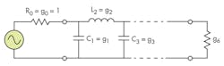
Figure 1 is a simple schematic diagram of the prototype Chebyshev lowpass filter. For the required passband ripple, Lar, in dB, and the minimum stopband attenuation, Las, in dB, at a stopband characteristic impedance of â¦s, in â¦, the degree of the prototype lowpass Chebyshev filter that will meet the required specifications can be found by Eq. 1:
n ≥ cosh-1{[(100.1Las – 1) /(100.1Las – 1)]0.5}/ cosh -1(â¦s) (1)
By assuming that the minimum stopband attenuation at â¦s = 2â¦cutoff = 2 and the passband ripple have been chosen as 50 dB and 3 dB, respectively, the degree of the Chebyshev lowpass prototype is calculated to be n = 5. The lowpass prototype parameters calculated from Eq. 1 are listed in the table.
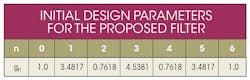
Figure 2 shows the general structure of a tapped combline filter. To design a combline BPF, the following parameters are also required: center passband frequency, F0, and passband bandwidth, BW. The filter is designed for a bandwidth (BW) of 100 MHz and a center frequency, F0, of 1,200 MHz.
To implement the proposed filter, quarter-wave transformers were used as impedance inverters. Using parameters gi calculated previously, it is possible to obtain the coupling coefficients of adjacent resonators Mi, i + 1 and the external quality factors (Qs) of the resonators at the inputs and outputs as1:
Mi, i + 1 = BW/F0( gigi+ 1)0.5, i = 1, 2, 3, 4 (2)
Qe1 = F0g0g1/BW, Qe5 = F0g5g6/BW (3)
From the above equations, M1,2 = M4,5 = 0.0511; M2,3 = M3,4 = 0.0448; and Qe1 = Qe5 = 41.7804. The prototype stripline combline filter was designed on a circuit laminate with relative dielectric constant of 3.38 and thickness of 0.98 mm (RO4003C material from Rogers Corp.). A line width was established at W = 0.55 mm with a line length of L = 20 mm and trace thickness t = µm for all the filter line elements except the terminating lines. The terminating lines were 0.93 mm wide, matching a terminating impedance of 50 â¦.
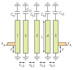
The coupling coefficient of the two adjacent resonators can be calculated by Eq. 41:
M = (F2H – F2L)/F2H + F2L (4)
where FH and FL represent the frequencies of the even- and odd-mode oscillations, respectively, in a system with two coupled resonators. These correspond to clearly pronounced peaks in the attenuation characteristic for the dual resonator circuit.
By changing the spacing between the resonators and calculating the coupling coefficient using Eq. 4, the design curve of the coupling coefficient versus spacing, s, can be obtained. The dimensions of the spacing required to achieve the design requirements for the resonant circuit for the design parameters can then be found from a curve of coupling coefficient versus s (Fig. 3) as: s1,2 = s4,5 = 0.45 mm and s2,3 = s3,4 = 0.53 mm.
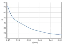
The external Q of the filter can also be extracted from Eq. 51:
Qe = ω0/(Δω±90°) (5)
where ω0 is the resonant frequency of the filter and Δω±90° is the absolute bandwidth between ±90-deg. points in the phase of S11. By changing the taping position y and calculating the external Q of the filter using Eq. 5, it is possible to generate a design curve of external filter Q versus y. With this curve (Fig. 4), the required taping position is obtained as y = 0.30 mm.
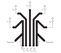
For tuning capability, varactor diodes were added to the proposed filter as variable capacitors, in place of the short-circuited end of the combline filter. Due to the small size of the proposed filter and fabrication issues involving small circuit dimensions, there is insufficient space to add varactor diodes in place of the short-circuited end of the coupling lines without interference. Therefore, the ends of the coupling lines are bent so that they do not interfere with each other once the varactor diodes have been added.
Figure 5 shows the modified structure of the combline filter after the coupling lines have been bending the end of the couple lines. A bending angle of 45 deg. was chosen for minimum impact on the design.
Sizing Up Simulations
The filter circuit’s performance possibilities were simulated with the Advanced Design System (ADS 2009) computer-aided-engineering (CAE) simulation software from Agilent Technologies (now Keysight Technologies). With the aid of the modeling software, the dimensions of the filter and the capacitance values were optimized with the following goals: the filter passband loss should be less than 2 dB and the filter stopband rejection should be more than 50 dB.
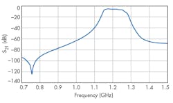
Figure 6 shows the simulated frequency response of the bandpass filter. As displayed in Fig. 6, the filter has a bandwidth of 100 MHz with center frequency (F0 of 1,200 MHz. The stopband rejection level and passband ripple of the filter are about 50 dB and 3 dB, respectively, which are in keeping with the design goals.
To demonstrate filtering tuning, a constant capacitance value (C) was added to the capacitance of each varactor diode; Fig. 7 shows the simulated filter frequency response for different values of C. As the plots show, by changing the capacitance of the varactor diodes, the center frequency of the filter can be tuned across a frequency range of 900 to 1,300 MHz with good impedance matching.
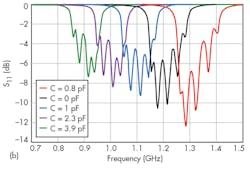
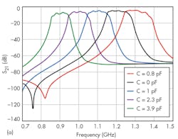
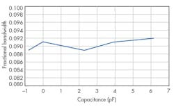
Figure 8 shows the filter’s fractional bandwidth as a function of C. The fractional bandwidth of the filter (about 9%) is very stable when tuning the center frequency, due to the constant coupling coefficient of adjacent resonators during tuning.
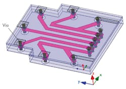
The simulation results were achieved using two-and-one-half-dimension (2.5D) ADS simulation tools. Although more time-consuming, a three-dimensional (3D) software solver was needed for greater simulation accuracy. But even a 3D solver may not properly predict the effects of certain circuit structures, such as viaholes. For improved accuracy, the High-Frequency Structure Simulator (HFSS) full-wave electromagnetic (EM) simulator from Ansys was used in the filter simulations. Figure 9 shows a 3D HFSS schematic diagram of the stripline combine BPF, with each viahole modeled as a cylindrical structure.
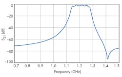
As Fig. 10 shows, the presence of viaholes will change the frequency response of the combline BPF. As an example, the 3D-modeled filter has a narrower transition band than simulations from the 2.5D ADS analysis. Still, the effects of the viaholes on filter frequency response are negligible, meaning that the 2.5D simulations are still valid and accurate.
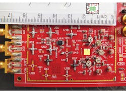
A hardware version of the filter was fabricated on RO4003C laminate using surface-mount-technology (SMT) packaged varactor diodes to provide the variable capacitances needed for filter passband tuning (Fig. 11). Unfortunately, these diodes contribute to the losses of the filter and, for some applications, an additional amplifier may be needed to compensate for undesirable passband losses.
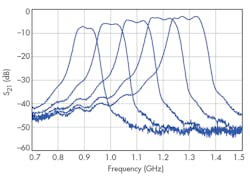
The filter was characterized (Fig. 12) with a model FSL6 spectrum analyzer from Rohde & Schwarz. The filter tuning range from 0.9 to 1.3 GHz had a nearly constant fractional bandwidth (about 9%). The rejection level at both upper and lower stopbands was about 50 dB, and measured passband ripple was about 3 dB. The frequency range and response measured with the spectrum analyzer was found to be quite similar to the performance predicted by the computer simulations.
Hossein Nikaein, Researcher
Farzad Zangeneh-Nejad, Researcher
Reza Safian, Engineer
Department of Electrical and Computer Engineering, Isfahan University of Technology, Isfahan, Iran 84156
References:
1. J.-S Hong and M.J. Lancaster, Microstrip Filters for RF/Microwave Applications, Wiley, New York, 2001.
2. C.B. Hofman and A.R. Baron, “Wideband ESM receiving systems-Part I,” Microwave Journal, Vol. 23, No. 9, September 1980.
3. G.L. Hey-Shipton, “Combline Filters for Microwave and Millimeter Wave Frequencies. Part 1,” Watkins-Johnson Company Tech-Notes, Vol. 17, September/October 1990, Watkins-Johnson Co., Palo Alto, CA.
4. G. L.Matthaei, “Comb-line Bandpass Filters of Narrow or Moderate Bandwidth,” Microwave Journal, August 1963, pp. 82-91.
5. C. Lugo and J. Papapolymerou, “Dual mode reconfigurable filter with asymmetrical transmission zeros and center frequency control,” IEEE Microwave & Wireless Component Letters, Vol. 16, No. 9, 2006, pp. 499-501.
6. J.-S Hong, ”Reconfigurable planar filters,” IEEE Microwave Magazine, Vol. 10, No. 6, 2009, pp. 73-83.
7. G.M. Rebeiz, I. Reines, M.A. El-Tanani et al., “Reconfigurable planar filters,” IEEE Microwave Magazine, Vol. 10, No. 6, 2009, pp. 55-72.
8. J. Nath, D. Ghosh, J.-P. Maria, A.I. Kingon, W. Fathelbab, P.D. Franzon, and M. B. Steer, “An electronically tunable microstrip bandpass filter using thin-film barium-strontium-titanate (BST) varactors,” IEEE Transactions on Microwave Theory & Techniques, Vol. 53, No. 9, 2005, pp. 2707-2712.
9. P.W. Wong and I.C. Hunter, “Electronically tunable filters,” IEEE Microwave Magazine, Vol. 10, No. 9, 2009, pp. 46-54.
10. I.C. Hunter and J.D. Rhodes, “Electronically tunable microwave bandpass filters,” IEEE Transactions on Microwave Theory & Techniques, Vol. 30, No. 9, 1982, pp. 1,354-1,360.
11. A.R. Brown and G.M. Rebeiz, “A varactor-tuned RF filter,” IEEE Transactions on Microwave Theory & Techniques, Vol. 48, No. 7, 2000, pp. 1,157-1,160.
12. J. Lee and K. Sarabandi, “An analytic design method for microstrip tunable filters,” IEEE Transactions on Microwave Theory & Techniques, Vol. 56, No. 7, 2008, pp. 1,699-1,706.
13. S.J. Park and G.M. Rebeiz, “Low-loss two-pole tunable filters with three different predefined bandwidth characteristics,” IEEE Transactions on Microwave Theory & Techniques, Vol. 56, No. 5, 2008, pp. 1,137-1,148.
14. M. Sanchez-Renedo, “High-selectivity tunable planar combline filter with source/load-multiresonators coupling,” IEEE Microwave & Wireless Components Letters, Vol. 17, No. 7, 2007, pp. 513-515.
15. B.W. Kim and S.W. Yan, “Varactor-Tuned Combline Bandpass Filter Using Step-Impedance Microstrip Lines,” IEEE Transactions on Microwave Theory & Techniques, Vol. 52, No. 4, 2004, pp. 1,279-1,283.
16. M.A. El-Tanani and G.M. Rebeiz, “A two-pole two-zero tunable filter with improved linearity,” IEEE Transactions on Microwave Theory & Techniques, Vol. 57, No. 4, 2009, pp. 830-839.
17. M.A. El-Tanani and G.M. Rebeiz, “High performance 1.5-2.5 GHz RF MEMS tunable filters for wireless applications,” IEEE Transactions on Microwave Theory & Techniques, Vol. 58, No. 6, 2010, pp. 1629-1637.
18. X.G. Wang, Y.H. Cho, and S.W. Yun, “A tunable combline bandpass filter loaded with series resonator,” IEEE Transactions on Microwave Theory & Techniques, Vol. 60, No. 6, 2012, pp. 1,569-1,576.
19. L. Athukorola and D. Budimir, “Compact second-order highly linear varactor-tuned dual-mode filters with constant bandwidth,” IEEE Transactions on Microwave Theory & Techniques, Vol. 59, No. 9, 2011, pp. 2,214-2,220.
20. H. Joshi, H.H. Sigmarsson, S. Moon, D. Peroulis, and W. J. Chappell, “High-performance fully reconfigurable tunable bandpass filter,” IEEE Transactions on Microwave Theory & Techniques, Vol. 57, No. 12, 2009, pp. 3,525-3,533.
21. A.C. Guyette, “Alternative architectures for narrowband varactor- tuned bandpass filters,” in Proceedings of the 2009 European Microwave Conference, September 2009, pp. 1,828-1,831.
Looking for parts? Go to SourceESB.
This file type includes high resolution graphics and schematics when applicable.
